Build The Data Foundation of Your Algo Trading Platform (in an afternoon)
Virgil
A pragmatic walkthrough: data model → seeded database → three core dashboards → two bonus sketches. Stocks-first, with a one-paragraph crypto adaptation at the end.
Why this post exists
Most "build an algo trading solution" tutorials fall to one of two extremes. Either they hand you a toy trades(symbol, price, qty) table that collapses the moment you ask "where's the strategy that placed it?" — or they march you through a 60-table OMS schema lifted from a sell-side bank that nobody actually needs to learn from.
This post sits in the middle. We're going to model an algorithmic trading data model — strategies, signals, orders, fills, positions, P&L — in 12 tables across 4 layers, seed it with realistic data, and put five dashboards on top. Everything runs on DataPallas. The data model is the part that actually matters; the rest is mechanics.
What this post is not claiming. This is not "a data model nobody else has". Open-source frameworks like NautilusTrader, freqtrade, zipline, backtesting.py, and vectorbt already model trades, orders, positions — some with richer schemas than the one here. So what's the point?
Three things:
Small enough to learn from. NautilusTrader's production schema is much larger — too much to internalise before lunch. Vectorbt keeps everything in-memory. Freqtrade is single-bot and crypto-first. The 12 tables here are deliberately fewer — sized to fit in your head in one sitting and serve as a scaffold for the model you'll end up writing.
The build your own dashboards approach. Schema → seeded database → operational dashboards, without writing a single line of frontend code. The data model is the vehicle; the dashboards workflow is what's being demonstrated end-to-end.
This model together with the dashboards are complementary to the frameworks (e.g. NautilusTrader), not a substitute. The frameworks execute strategies. The model + dashboards here observe them — across runs, across versions, across strategies.
Point any framework's output at a schema like this and you get operational dashboards none of them ship.
What this post IS NOT
This post is not a "do exactly this and you'll get results" recipe.
Read it as a (re)learning exercise — an opportunity to think once more about the shape of an algo trading platform's data, and to compare that shape against the one you already have (or the one you're about to build).
If, after that thinking exercise, you come up with your own data model — one that doesn't look like the 12 tables here but is intentional and makes sense for your use case — that's exactly the right outcome. Go build your own custom, specific data model. The 12 tables here are a reference to think against, not a template to copy.
Docker Engine — DataPallas needs Docker to spin up the TimescaleDB starter pack.
That's it. No broker account, no market data subscription, no Python algo framework. We're modelling the data platform, not running money.
A quick word on TimescaleDB
The whole thing runs on TimescaleDB, which is the database DataPallas spins up for you. Two things worth knowing:
It's PostgreSQL with an extension — same engine, same SQL, same drivers, same tooling. Anything that talks to Postgres talks to TimescaleDB. The extension adds time-series superpowers on top of vanilla Postgres; it doesn't replace it.
It's built for time-series workloads — append-only data, time-range queries, automatic partitioning by time, and built-in rollups (called continuous aggregates). That's exactly the shape of market data: bars arrive every minute, they never get updated, and every dashboard query filters by a time window.
In this post, only one table — bar_1m — actually uses the TimescaleDB-specific machinery (it's declared as a hypertable, and the 5-minute / hourly / daily bars are continuous aggregates rolled up from it). The other eleven tables are plain Postgres. If you ever needed to lift this schema onto vanilla Postgres, you'd lose the time-series performance on bars but everything else would work unchanged.
Going further — crypto adaptation, tick-level upgrade, where the design grows next
Quick terminology
A few words to pin down before we go further. These trip people up.
Bar (or candle): one row of OHLCV data — Open, High, Low, Close, Volume — covering a fixed time window.
Intraday: any resolution finer than one trading day. We'll use 1-minute bars as our raw grain. One US stock generates ~390 1-minute bars per trading day (6.5 hours × 60 minutes).
Tick: every individual trade or quote update. Far heavier than bars; we are not going there in this post (see Going further for when you should).
Algo / strategy: a piece of code that reads market data, emits signals, and decides whether to send orders.
Signal: the algo's output ("I think we should buy AAPL"). Not the same as an order — a signal can be ignored by risk layers, throttled, or batched.
Order: an instruction sent to a venue or broker.
Fill (or execution): a confirmation back from the venue that part or all of the order traded. One order can have many fills.
Position: how much of an instrument you currently hold. Derived from fills.
P&L: profit and loss. Realized P&L locks in when you close a position; unrealized P&L floats with the market price of open positions.
Everything below builds on those nine words.
4 layers, 12 tables
The single most useful mental model for an algo trading platform is four concentric layers. Reference data on the outside; analytics on the inside; everything else flows between.
Twelve tables. That's it. Get the layers right and every later question — "where do I store this?", "is this a primary or derived table?", "how do I isolate a backtest from live trading?" — has an obvious answer.
Boring on purpose. Mostly INSERT-once, UPDATE-rarely. Notice strategy.params_schema_json — that's a JSON Schema describing what parameters the algo accepts (e.g. {"lookback": {"type": "int", "default": 20}}). The schema lives here; concrete values live on strategy_run (Layer 3). This split is what makes backtests reproducible.
This is the only raw market-data table. It is also the only TimescaleDB hypertable. 5-minute, hourly, and daily bars are not separate tables — they are continuous aggregates rolled up automatically:
CREATE MATERIALIZED VIEW bar_5mWITH (timescaledb.continuous) ASSELECT instrument_id, time_bucket('5 minutes', ts) AS ts, first(open, ts) AS open, max(high) AS high, min(low) AS low, last(close, ts) AS close, sum(volume) AS volume, sum(close * volume) / nullif(sum(volume), 0) AS vwap, sum(trade_count) AS trade_countFROM bar_1mGROUP BY instrument_id, 1;
Same shape for bar_1h and bar_1d. Never store the same bar at two resolutions. Storage doubles, and the moment a vendor sends you a 1-minute correction at 14:32, your 5-minute bar is silently wrong until something refreshes it. Continuous aggregates handle that for you.
Data volume check: 30 instruments × ~64 trading days (90 calendar days minus weekends) × 390 bars/day ≈ 750k rows. Comfortable on any laptop.
The shape that matters is strategy_run → signal → order → fill. A run emits signals; signals (sometimes) become orders; orders generate one or more fills.
Hard rules:
Append only. Never UPDATE a fill. If the broker corrects one, insert a compensating fill.
Every algo-emitted row carries strategy_run_id. This single FK lets you isolate a backtest from paper from live trading. Drop it and you will be reconstructing which fill belongs to which run from timestamps for the rest of your life.
position is derived. The truth lives in fills. Materialize position with a view and refresh it on a schedule (or trigger). Don't let humans or algos write to it directly.
A snippet for the position view:
CREATE VIEW position_now ASSELECT sr.account_id, o.instrument_id, sum(case when f.qty_signed > 0 then f.qty_signed else 0 end) AS long_qty, sum(case when f.qty_signed < 0 then f.qty_signed else 0 end) AS short_qty, sum(f.qty_signed) AS net_qty, sum(f.qty_signed * f.price) / nullif(sum(f.qty_signed), 0) AS avg_costFROM fill fJOIN "order" o ON o.id = f.order_idJOIN strategy_run sr ON sr.id = o.strategy_run_idGROUP BY 1, 2HAVING sum(f.qty_signed) <> 0;
(qty_signed = qty * sign(side) — store it as a generated column on fill for sanity.)
trade is the round-trip table — one row per "open a position, close a position" cycle. Almost every dashboard query in the Dashboards section reads from this table, not from fill. Building it is a SQL exercise: pair each closing fill with the matching opening fill (FIFO or LIFO; pick one and document it).
equity_curve is the per-strategy mark-to-market over time. Generate one row per minute (or per bar, or per fill — your call). This is what feeds the equity-curve chart everyone wants to see first.
Crypto adaptation (one paragraph)
Three tweaks. Replace exchange.mic with exchange.code (Binance and Coinbase have no MIC code). Add quote_currency to instrument so BTC/USDT and BTC/USD are distinct rows. Drop lot_size enforcement (most crypto venues accept arbitrary precision). Everything else — every layer, every rule, every dashboard — works unchanged.
Standing it up with DataPallas
Three steps, no surprises.
Step 1 — Spin up the TimescaleDB starter pack.
On DataPallas's main screen, open the Explore Data & Build Dashboards tab and click Explore More Apps That Go Well Together with DataPallas. The Apps screen opens — switch to the Starter Packs tab next to Apps, find TimescaleDB, and click Start. The pack boots a Postgres 16 + Timescale container on port 5433. First boot takes ~30–60s while Docker pulls the image; warm starts are faster.
Once started, open Configuration → Connections → New → Database and create a new TimescaleDB connection pointing at localhost:5433 (default credentials: postgres/postgres, database postgres). Click Test DB Connection and confirm the prompt.
Click Yes → you should see the green App status: great, no errors, no warnings chip. The connection is ready.
One database server (one starter pack), not two. TimescaleDB is PostgreSQL with an extension — same server, same connection, same SQL.
Let's use the Seed Data tab to create our sample schema along with some sample data to work with. Paste the trading-platform seed script into the editor.
The script does, in order:
Creates the 12 tables, the hypertable on bar_1m, the three continuous aggregates, and the position_now / equity_curve views.
Inserts ~30 instruments across 4 sectors on NYSE and NASDAQ.
Generates 90 days of synthetic 1-minute OHLCV per instrument with a believable random-walk drift and intraday volatility shape (open/close volume bumps).
Wait a few minutes for the data to be generated — it produces a good amount of data which will let us build useful dashboards on top of it. When it finishes you have a fully populated algo trading database.
When the database seeding script is done, open CloudBeaver (setup details below) and run this sanity query:
SELECT
  (SELECT count(*) FROM instrument)            AS instruments,
  (SELECT count(*) FROM bar_1m)                AS bars,
  (SELECT count(*) FROM strategy_run)          AS runs,
  (SELECT count(*) FROM signal)                AS signals,
  (SELECT count(*) FROM fill)                  AS fills,
  (SELECT count(*) FROM trade)                 AS round_trips;
You should see roughly: 30 / 750k / 200 / 13k / 8k / 3.9k. (Bar count is calendar-days × 5/7 because weekends are skipped — real markets are closed Sat/Sun.)
CloudBeaver — for ad-hoc queries against TimescaleDB
CloudBeaver describes itself as "the professional data management software trusted by experts" — a web-based database management tool in the same family as SQL Server Management Studio (for SQL Server) or MySQL Workbench (for MySQL).
DataPallas ships a CloudBeaver app (community-edition database browser) you can spin up alongside it for ad-hoc SQL and schema inspection. On DataPallas's main screen, open the Explore Data & Build Dashboards tab and click Explore More Apps That Go Well Together with DataPallas — that opens the full Apps list. Find the CloudBeaver row, click Start, then Launch once it's running. Same one-click lifecycle as every other app in this post.
While you're on that screen, the Starter Packs tab — where TimescaleDB and other sample databases live — sits right next to Apps. One more click and you're there.
Once CloudBeaver opens, create a new PostgreSQL connection with these details:
Field
Value
Host
host.docker.internal
Port
5433
Database
postgres
Username
postgres
Password
postgres
Why host.docker.internal and not localhost? CloudBeaver and the TimescaleDB starter pack each run in their own Docker container, on separate Docker networks. Inside the CloudBeaver container, localhost resolves to the CloudBeaver container itself — not to the host machine where TimescaleDB's port 5433 is exposed. host.docker.internal is Docker Desktop's special DNS name that resolves to the host machine, so CloudBeaver reaches the host's :5433, which Docker then forwards into the TimescaleDB container.
A note on writing SQL and scripts
If you already know SQL or scripting — lucky you, it'll come in handy as we go.
For everyone else who isn't comfortable writing SQL or scripts: DataPallas puts a Hey AI, Help Me… button right next to every editor where SQL or a script is expected.
✦
Hey AI, Help Me…
Click it, get a feel for how it works, and in a couple of minutes you'll be writing the SQL and scripts you need like an expert. :-)
Dashboards (3 mandatory, 2 bonus)
Three core dashboards cover 90% of what you'll actually look at every day. Together they answer the three questions every algo trader needs answered every single day — does it work?, what am I holding right now?, and am I getting filled at the prices I expect? — and without any one of them you're flying blind on a dimension that can quietly ruin you.
Dashboard 1 — Strategy Performance is the does it work? dashboard: P&L, Sharpe, drawdown, win rate across every strategy run — the scorecard that tells you which algos to scale, which to kill, and which to send back to research.
Dashboard 2 — Live Positions & Exposure is the what am I holding right now? dashboard: gross / net exposure, leverage, per-symbol positions and sector breakdown — the view you watch during market hours to make sure you're inside risk limits.
Dashboard 3 — Execution Quality is the am I getting filled at the prices I expect? dashboard: signal-to-fill latency, fill rate, slippage histogram — the one that catches broker / venue degradation before it quietly erodes the P&L the other two dashboards report.
Stick around for two bonus dashboards with full widget specs (layout, SQL, chart bindings — no live screenshots, so you build them yourself): Trade Journal (per-round-trip P&L distribution + MFE/MAE scatter, for human review) and Market Data Health (bar gaps, stale-last-bar age — the unsexy one that prevents silent disasters).
Start the Explore Data & Build Dashboards app
Before you can build any dashboard, the Explore Data & Build Dashboards app needs to be running. On DataPallas's main screen, click the Explore Data & Build Dashboards tab — the app card with a Start button is right there. Click Start, wait until the state flips from Starting to running, then click Launch to open the canvas builder.
Notice the list of dashboards below the app card. That's where every dashboard you build and publish from this point on will show up — bookmark this screen and you'll always have a one-click way back to any of them.
Dashboard 1 — Strategy Performance
The does it work? dashboard — and the one everyone wants on day one.
Equity curve per strategy — line chart, time-bucketed from equity_curve, one series per strategy_run_id. The equity curve is the single most important chart in trading: it shows account value over time. A healthy algo trends up-and-to-the-right with shallow dips; comparing strategies side-by-side here tells you which one to scale and which to retire.
Drawdown ribbon underneath, shaded red where drawdown_pct < 0. Drawdown is how far you've fallen from your last peak. Traders care about it more than P&L because it sets the psychological and risk-budget pain threshold — a strategy with great returns but a 40% drawdown is one nobody can actually stomach.
KPI tiles across the top: Sharpe ratio, win rate, profit factor, total trades, max drawdown, average holding period. These six numbers are the standard "scorecard" traders use to judge a strategy at a glance — risk-adjusted return (Sharpe), how often it's right (win rate), how much winners pay vs. losers (profit factor), sample size (trades), worst-case pain (max DD), and trade tempo (holding period).
Filters: strategy, run mode (backtest / paper / live), date range, account. Same dashboard, three lenses. Backtests look great on paper; paper trading proves the code actually runs; live is the only number that pays the bills. The filter lets one dashboard answer "does this still work?" across all three stages.
Headline query for the equity curve:
SELECT time_bucket('1 day', ts) AS day, strategy_run_id, avg(equity) AS avg_equityFROM equity_curveWHERE strategy_run_id IN (1, 5, 10, 50, 100)GROUP BY 1, 2ORDER BY 1, 2;
Our goal is to end up with a dashboard that looks roughly like this — a title block, a Strategy Runs filter, six KPI tiles across the top, then the Equity Curve and Drawdown Ribbon charts stacked underneath:
The sketch above shows the dashboard with five strategy runs picked in the filter chip (Run 1, 5, 10, 50, 100) — every KPI and chart below redraws for just those runs, and each run gets its own colour-coded line in the Equity Curve and area band in the Drawdown Ribbon. The default state of the dashboard is * (no filter, all 200 runs aggregated together); the Strategy Runs chip at the top is the lever to narrow it down — open it, tick one run or pick a handful, and every widget rebinds to that selection.
Building Dashboard 1 — step by step
This is a hands-on tutorial. You'll click through DataPallas's Explore Data canvas widget by widget and end up with a 9-component dashboard (title + parameter + 6 KPIs + 2 charts). Some widgets you'll configure visually only — no code; others need a bit of SQL. Don't freak out: DataPallas has a beautiful AI integration built right into every SQL/script editor (the Hey AI, Help Me… button we met earlier) — the AI drafts the SQL and you reap the benefits. :-) Six phases — the order below is the order the dashboard visibly grows as you scroll through this post:
#
Phase
What you add
1
Title block
Text block at the top
2
Strategy Runs multi-select parameter
The dashboard filter that lets the viewer pick which strategy runs to show
3
KPI tiles row
6 small Number widgets: Total P&L, Total Trades, Max DD, Best Trade, Win Rate, Sharpe
4
Equity Curve
Line chart from equity_curve, AVG equity grouped by run
5
Drawdown Ribbon
Area chart from equity_curve, AVG drawdown_pct grouped by run
6
Layout polish + publish
Resize, arrange, verify, publish
Each phase produces a visible win and teaches one new DataPallas concept. Total time: ~40 minutes if you've never touched the canvas before.
Why parameter first, then widgets — not the other way around? Each KPI/chart we add binds to ${strategy_runs} from the moment it's created. Defining the parameter once at the top means we don't have to revisit every widget at the end to wire up the filter — the binding happens inline as the widget is built.
Phase 1 — Title block
Goal: create the dashboard, name it, drop a heading text block.
In DataPallas's top nav, click Explore Data.
Create a new canvas. The canvas opens with title "Untitled Canvas" at the top.
Click the canvas title and rename it to Algo Trader — Strategy Performance.
In the left Data Source panel, the connection dropdown should already show your TimescaleDB connection — for this tutorial: db-algotrader-db-timescaledb. If not, pick it from the dropdown.
Click the UI Elements tab on the left (next to Data Source).
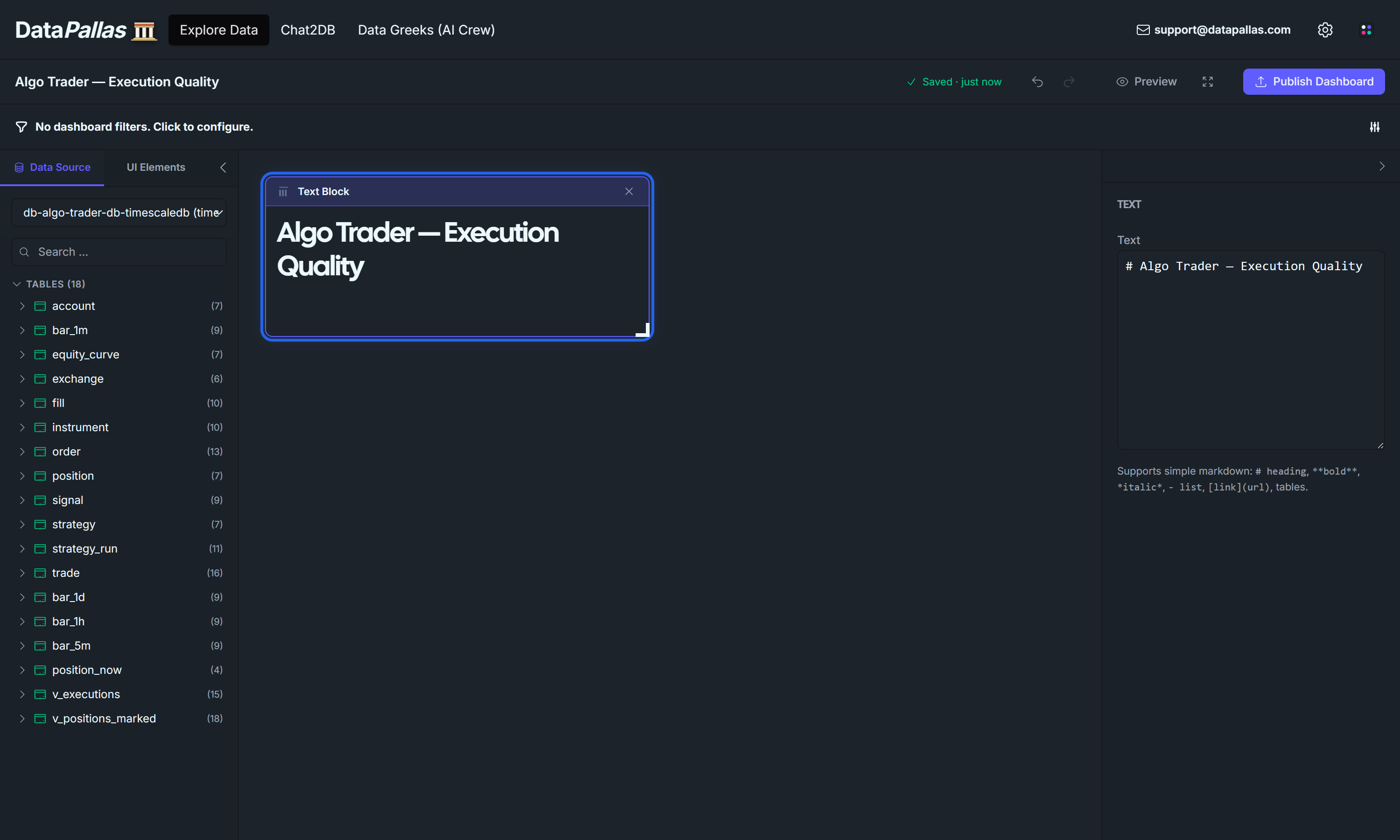
Drag a Text Block widget onto the canvas, near the top.
With the text block selected, the right configuration panel reveals a Text input. Type:
# Algo Trader — Strategy Performance
Phase 2 — Strategy Runs multi-select parameter
Goal: define one canvas parameter at the very top — Strategy Runs — that every data widget we add next will bind to via the ${strategy_runs} placeholder. Doing this before the data widgets means each KPI/chart can be created with the filter already in place; we don't have to revisit them later.
At the top of the canvas, click the small gear icon in the top-right corner of the parameter row (the empty band just above the first widget).
The "Dashboard Filters" dialog opens. Click Add parameter:
Name:Strategy Runs
Type:String (the dropdown shows String / Number / Date / Boolean)
Default value:* — the wildcard, meaning "no filter, show all strategy runs". The dashboard opens with this default, so first-time viewers see the aggregated totals before they narrow down.
UI control:multiselect — dropdown with checkboxes. Options come from a SQL query that returns two columns: (id, label). The dropdown shows the friendly label (e.g. mean_reversion_5m #1 (backtest)), the IN-list binds only the raw id. Query: SELECT sr.id, s.name || ' #' || sr.id || ' (' || sr.mode || ')' AS label FROM strategy_run sr JOIN strategy s ON s.id = sr.strategy_id ORDER BY sr.id.
Page size:5 — paginate the dropdown 5 runs at a time so the picker stays manageable as runs accumulate.
The Parameter ID below the name auto-fills as strategy_runs. Confirm it has an underscore, not a hyphen. If you see strategy-runs, your DataPallas predates v15.2 — the hyphen breaks the JDBI named-parameter parser downstream.
Click I'm Done.
Dashboard Filters dialog — DSL mode. Prefer typing to clicking? Toggle the dialog into DSL mode and paste this block instead of filling the fields by hand:
reportParameters { parameter(id: 'strategy_runs', type: String, label: 'Strategy Runs', defaultValue: '*') { constraints(required: false) ui(control: 'multiselect', options: "SELECT sr.id, s.name || ' #' || sr.id || ' (' || sr.mode || ')' AS label FROM strategy_run sr JOIN strategy s ON s.id = sr.strategy_id ORDER BY sr.id", pageSize: 5) }}
Click I'm Done. The param now appears as a multi-select chip at the top of the canvas, defaulting to All.
Why * as the default and not the first 5 runs? With * (= "no filter") every widget we add next renders the unfiltered totals — Total P&L across all 200 runs, all 3,884 trades, etc. The viewer can narrow down later by typing into the chip. If you'd rather pre-narrow, set the default to e.g. 1, 5, 10, 50, 100.
Phase 3 — KPI tiles row
Goal: add 6 single-value Number widgets — Total P&L, Total Trades, Max Drawdown, Best Trade, Win Rate, Sharpe Ratio. Four are UI-only Summarize; two require the Finetune tab in SQL mode. Each widget binds to ${strategy_runs} from creation.
The lesson here is when to drop into SQL. The UI-only Summarize panel handles single aggregations on a single column (COUNT, MIN, MAX, AVG, SUM). It can't express:
Conditional aggregations (SUM(CASE WHEN ... THEN 1 ELSE 0 END))
Ratios of two aggregates (wins / total)
Window-function calculations (LAG(), STDDEV() over a partition)
When you need any of those, drop into Finetune → SQL editor and write the raw query.
3.1 — Total P&L (UI configuration only, currency format)
The headline KPI: did this strategy actually make money? Drag this one first — the leftmost spot in the KPI row.
Drag trade onto the canvas.
Right panel → Data tab → Summarize + → set the row to SUM of net_pnl.
Filter + → column: strategy_run_id, operator: in, click the ${} chip → pick ${strategy_runs}.
Click Run Query.
VISUALIZE AS → Number.
Display tab:
Format: Currency ($1,234).
Label: Total P&L.
trade.net_pnl is the per-closed-round-trip P&L the seed script wrote at trade close. Summing across rows gives total realized P&L for whatever runs the parameter is currently selecting (* = all 200 runs by default).
Expected with default *: ~$432,000.
Display tab — set:
Visualize As: Number
Label: Total P&L
Format: Currency ($1,234)
3.2 — Total Trades (UI configuration only)
Drag trade onto the canvas.
Summarize + → COUNT of id.
Filter + → strategy_run_idin → ${strategy_runs}.
Click Run Query.
VISUALIZE AS → Number.
Display tab → Label: Total Trades.
Expected with default *: ~3,467.
Display tab — set:
Visualize As: Number
Label: Total Trades
Format: leave as default Number (no decimals)
3.3 — Max Drawdown (UI configuration only, percent format)
Drag equity_curve onto the canvas.
Summarize + → MIN of drawdown_pct.
Filter + → strategy_run_idin → ${strategy_runs}.
Click Run Query.
VISUALIZE AS → Number.
Display tab:
Format: Percent (73.1%) — the widget multiplies by 100 and renders 1-2 decimals.
Label: Max Drawdown.
Expected with default *: ~-26.09% (worst per-day drawdown across all runs).
Display tab — set:
Visualize As: Number
Label: Max Drawdown
Format: Percent (12.3%)
3.4 — Best Trade (UI configuration only, currency format)
Drag trade onto the canvas.
Summarize + → MAX of net_pnl.
Filter + → strategy_run_idin → ${strategy_runs}.
Click Run Query.
VISUALIZE AS → Number.
Display tab:
Format: Currency ($1,234).
Label: Best Trade.
Expected with default *: ~$13,135.
Display tab — set:
Visualize As: Number
Label: Best Trade
Format: Currency ($1,234)
3.5 — Win Rate (Finetune SQL)
The Summarize UI cannot express "fraction of trades where net_pnl > 0" because it requires a CASE WHEN aggregate divided by COUNT(*). Open the Finetune tab and switch its mode to SQL.
Drag trade onto the canvas.
Right panel → click the Finetune sub-tab (next to Visual). The SQL editor appears.
Paste:
SELECT SUM(CASE WHEN net_pnl > 0 THEN 1 ELSE 0 END)::numeric / NULLIF(COUNT(*), 0) AS win_rate_pctFROM tradeWHERE strategy_run_id IN (${strategy_runs});
VISUALIZE AS → Number.
Click Run Query.
Display tab:
Format: Percent (73.1%) — the SQL returns a raw fraction (~0.55); the Percent formatter renders it as ~55%.
Label: Win Rate %.
Expected with default *: ~54.92% — close to a random-walk for our synthetic seed.
Note the parens around ${strategy_runs} — the placeholder goes insideIN ( ... ). The backend regex looks for that exact pattern to know it should bind a list rather than a scalar.
Display tab — set:
Visualize As: Number
Label: Win Rate %
Format: Percent (12.3%)
Why a raw fraction and not a pre-multiplied percentage. Pick one convention and stick with it: either emit 0.55 and use Percent format, OR emit 55 and use Number format. Don't mix — 100.0 * SUM(...) (returning 55) combined with Percent format gives you 5500% because the formatter multiplies by 100 again.
3.6 — Sharpe Ratio (Finetune SQL with window functions)
WITH daily_returns AS ( SELECT strategy_run_id, ts, (equity / NULLIF(LAG(equity) OVER (PARTITION BY strategy_run_id ORDER BY ts), 0)) - 1 AS daily_return FROM equity_curve WHERE strategy_run_id IN (${strategy_runs}))SELECT ROUND( ((AVG(daily_return) / NULLIF(STDDEV(daily_return), 0)) * SQRT(252))::numeric, 2) AS sharpe_ratioFROM daily_returnsWHERE daily_return IS NOT NULL;
VISUALIZE AS → Number.
Click Run Query.
Display tab:
Format: Number (1,234).
Label: Sharpe Ratio.
Expected somewhere between -0.5 and +1.0 for our random-walk seed (default * shows ~0.46). A real strategy with edge would show 1.5-2.0+; institutional benchmarks target 2-3+.
Display tab — set:
Visualize As: Number
Label: Sharpe Ratio
Format: Number (1,234) (2 decimals will be applied by the SQL itself)
Postgres ROUND() quirk worth knowing. PostgreSQL doesn't have ROUND(double precision, integer) — only ROUND(numeric, integer). The arithmetic above produces double precision because of the division and the SQRT() call, so a ::numeric cast is required before passing to ROUND. Other databases (MySQL, SQLite, ClickHouse) accept ROUND(double, int) natively, so this gotcha is Postgres-specific.
Phase 4 — Equity Curve (line chart)
Goal: add a line chart showing average equity over time, one series per strategy_run_id.
Click an empty area on the canvas to deselect any current widget.
Make sure the Data Source tab is active on the left.
Drag equity_curve onto the canvas (in the empty area below the KPI row). A Data Table widget appears showing raw rows — that's normal.
Look at the right panel. Under VISUALIZE AS the suggested widgets are Table / Detail / Number — DataPallas suggests these because we have no aggregation yet. We'll fix that next.
Click Summarize + in the right panel:
Click the COUNT dropdown → select AVG.
Click the strategy_run_id dropdown → select equity.
The row should now read: AVG of equity.
Under "Group by:", click the ts chip → bucket: Day. Click the strategy_run_id chip → bin: Don't bin.
Filter + → column: strategy_run_id, operator: in, click the ${} chip → pick ${strategy_runs}.
Sort + → column: ts, order: ASC.
Limit → change 500 to 10000 (the equity_curve table has more rows than 500 across all runs).
Display tab → Chart type → Line.
Click Run Query.
What you should see: one line per run currently selected by the parameter — defaulting to all 200 with *. If it looks like a tangled mess, that's because we wired the dashboard to show every run by default — it'll look beautiful the moment the viewer picks a handful of strategies from the filter. :-)
Display tab — set:
Visualize As: Chart
Chart Type: Line
Title: Equity Curve
Phase 5 — Drawdown Ribbon (area chart)
Goal: add a second chart underneath the equity curve, plotting each run's drawdown_pct over time. Same data source, different Y axis, area-style visualization. Together with the equity chart this tells the full performance + risk story.
Click an empty area on the canvas to deselect.
Drag equity_curve from the table list onto the canvas, dropping it in the empty area below the equity chart.
Group by: ts chip → bucket Day. strategy_run_id chip → bin Don't bin.
Filter + → strategy_run_idin → ${strategy_runs}.
Sort + → ts ASC. Limit → 10000.
Display tab → Chart type → Area. (Area is more appropriate than Line for drawdown — the shaded fill below zero visually communicates "loss territory".)
Click Run Query.
What you should see: a chart below the equity curve, X-axis dates matching the equity chart, Y-axis going from 0 down to negative values (e.g., 0 to -0.30 = 0% to -30% drawdown). Coloured downward spikes where any of the runs dipped below their prior peak. The 0-line at the top is the shape's ceiling — you can never have positive drawdown by definition.
Display tab — set:
Visualize As: Chart
Chart Type: Area
Title: Drawdown Ribbon
Phase 6 — Layout polish, verify, publish
Goal: rearrange the 9 widgets so the dashboard reads top-to-bottom like a real product surface, verify the parameter wires through, then publish.
Recommended layout — title row, KPI row across the top, two charts stacked beneath:
How to do it:
Drag widgets to reorder. Click and hold the widget's header strip (where it says # Number or 📊 Chart), drag it to the target slot, drop. The other widgets reflow around it.
Resize via the bottom-right corner. Hover the corner — a small triangle handle appears. Drag inward / outward. Number widgets are roughly the same size except Total P&L (slightly wider — $432,409 is 8 chars) and Sharpe Ratio (slightly narrower — 0.46 is 4 chars). Charts span the full canvas width.
Let widgets snap to the grid. The canvas has an invisible 12-column grid; widgets snap to it. Don't pixel-tweak — line them up by using grid columns (e.g. P&L = 3 cols, the four middle KPIs = 2 cols each, Sharpe = 1 col → sums to 12).
Verify the round-trip. Click the Strategy Runs chip and pick e.g. 1 only. Watch every widget redraw: charts collapse to a single series, KPI tiles snap to single-run values. Pick a few runs (1, 5, 10) → all 8 data widgets redraw with 3 runs of data. Pick All again → unfiltered totals return.
Publish. Click Publish Dashboard in the top-right. The canvas becomes a permanent URL you can bookmark, share, or embed — and the Strategy Runs parameter survives as an editable input on the published page too.
The published page isn't read-only — the Strategy Runs parameter at the top is interactive. Open the multi-select, Select None, tick a single run (e.g. 1), click OK, then Reload, then Yes in the confirm prompt. Every widget bound to ${strategy_runs} re-runs with the new selection and the page rebuilds in place — overlapping series collapse to one clean line, and the KPI tiles update to that single run's numbers:
Wow… you just shipped your first algo trading dashboard — and, if you think about it, nothing along the way was that hard, so there's really nothing stopping you from building your own.
Take a well-deserved 10-minute break, grab a coffee, then let's move on to building the next dashboard.
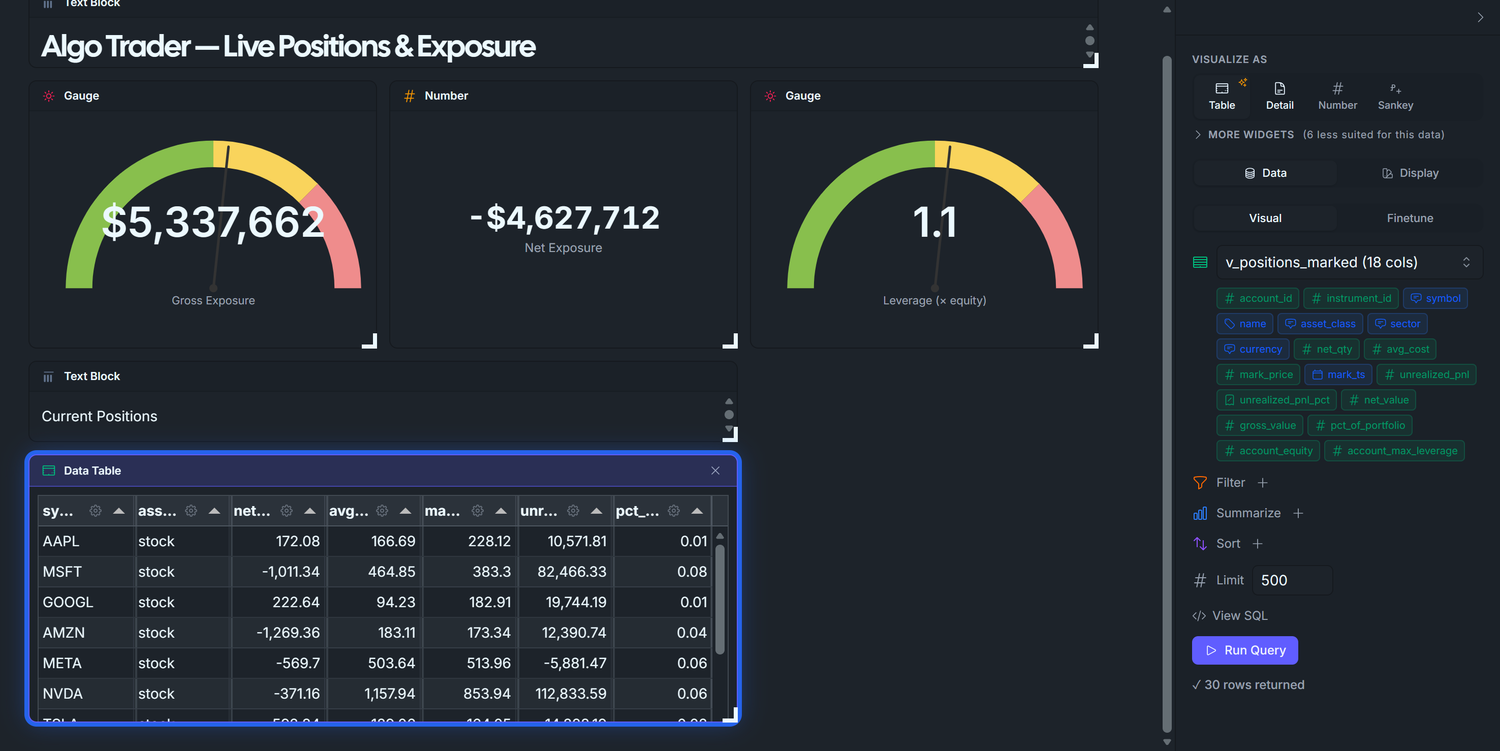
Dashboard 2 — Live Positions & Exposure
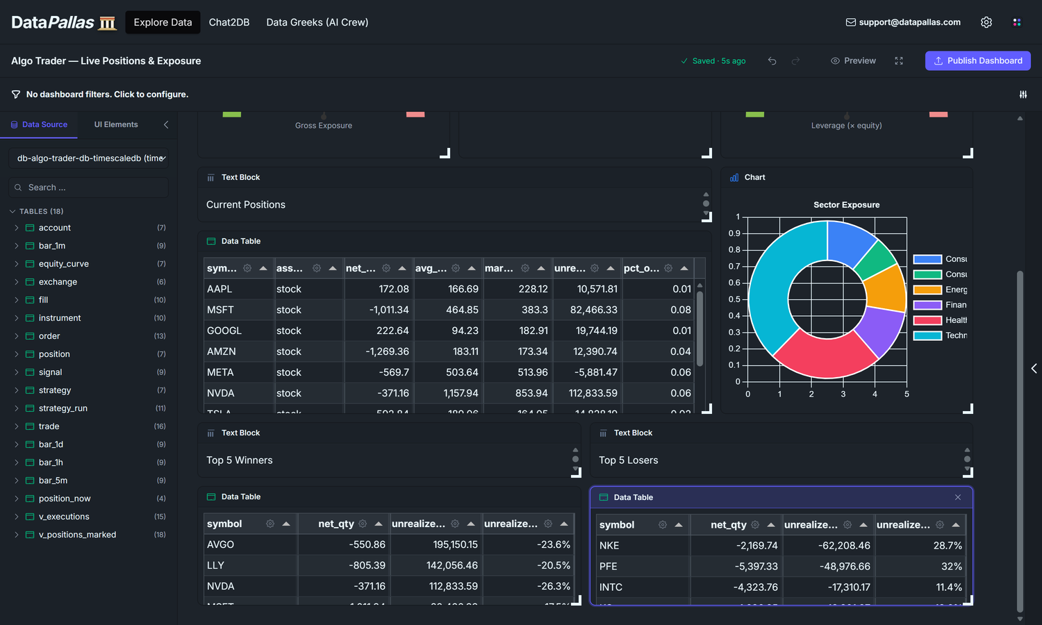
The what am I holding right now? dashboard — gross / net exposure, leverage, per-symbol positions. The view you watch during market hours.
Our goal is to end up with a dashboard that looks roughly like this — three KPI tiles (Gross / Net / Leverage) across the top, the Current Positions table next to a Sector Exposure donut, then Top 5 Winners and Top 5 Losers side-by-side:
D1 answered does the strategy work? over time. D2 answers a sharper, more immediate question: given the book I'm sitting on right now, can I survive a bad day? Three numbers carry that answer:
Gross exposure — the absolute dollar value of every position, summed. If the market dropped 10% tomorrow, this is roughly the dollar hit you'd take.
Net exposure — long sum minus short sum. Positive = a market rally helps you; negative = a market sell-off helps you; near-zero = market-neutral.
Leverage — gross divided by account equity. At 1× a 50% drawdown wipes the account; at 2× a 25% drawdown does it; at 4× a routine bad week ends the strategy.
Four widgets answer those three questions and then drill down to which symbol is driving it:
Three gauges (Gross · Net · Leverage) — half-circle dials with green/yellow/red bands sized to your account ceiling. Glanceable on purpose: needle in green = move on; yellow or red = drill into the table below to see which positions to trim.
Current Positions table — position_now joined to the latest bar_1m close: symbol, signed qty (+ = long, − = short), avg_cost, current mark, unrealized_pnl, pct_of_portfolio. The ledger. When a gauge above moves, this is the table that tells you which row caused it.
Sector Exposure donut — gross_value summed by instrument.sector. Concentration risk. A book that looks safe on the aggregate gauges can still take outsized damage if 60% of it sits in one sector — a FAANG sell-off or banking-sector wobble takes the whole book down. The donut tells you whether the book is spread thin enough that no single sector can sink you.
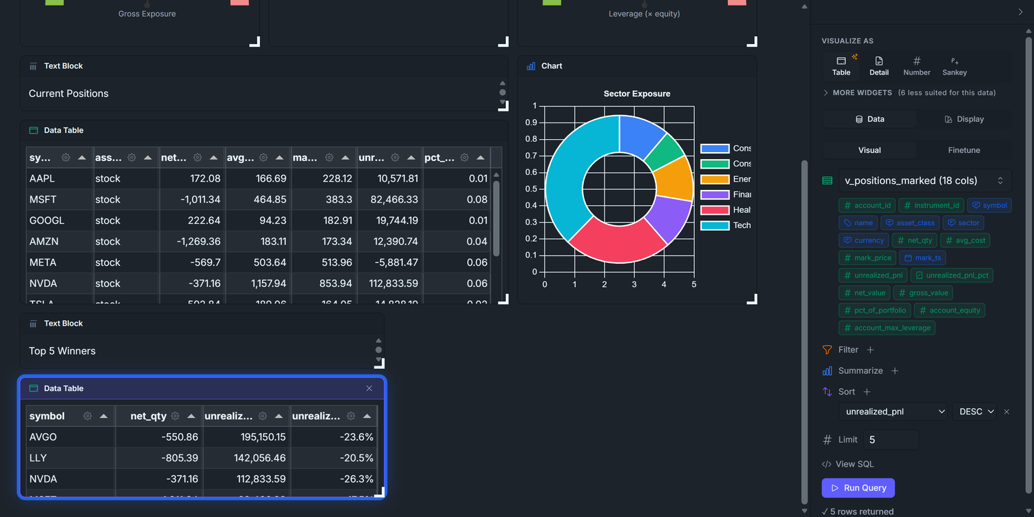
Top 5 Winners / Losers — biggest unrealized P&L moves since the positions opened. Twenty rows in the positions table are too many for the eye to triage. These two lists answer "what's making money, what's losing money" in two seconds — use them to pick which winners to trim and which losers to cut.
All four want the same join: positions × latest tick × instrument metadata × account equity. Rather than write that join four times in widget-level Finetune SQL, we define one denormalized view and let every widget target it via the visual builder. One piece of SQL, four visual-builder widgets.
Phase 1 — Define the base view v_positions_marked(the seed script already created this view for you — nothing to run here, just read through so you understand what the next widgets bind to)
This view is the single piece of SQL on the dashboard. The rest is point-and-click.
CREATE OR REPLACE VIEW v_positions_marked ASWITH latest_bar AS ( SELECT DISTINCT ON (instrument_id) instrument_id, ts AS mark_ts, close AS mark_price FROM bar_1m ORDER BY instrument_id, ts DESC)SELECT pn.account_id, pn.instrument_id, i.symbol, i.name, i.asset_class, i.sector, i.currency, pn.net_qty, pn.avg_cost, lb.mark_price, lb.mark_ts, (lb.mark_price - pn.avg_cost) * pn.net_qty AS unrealized_pnl, CASE WHEN pn.avg_cost <> 0 THEN (lb.mark_price - pn.avg_cost) / pn.avg_cost ELSE NULL END AS unrealized_pnl_pct, pn.net_qty * lb.mark_price AS net_value, -- signed (long +, short −) abs(pn.net_qty) * lb.mark_price AS gross_value, -- absolute (no sign) abs(pn.net_qty * lb.mark_price) / NULLIF(a.equity, 0) AS pct_of_portfolio, a.equity AS account_equity, a.max_leverage AS account_max_leverageFROM position_now pnJOIN latest_bar lb ON lb.instrument_id = pn.instrument_idJOIN instrument i ON i.id = pn.instrument_idJOIN account a ON a.id = pn.account_id;
A few design choices worth noting:
DISTINCT ON (instrument_id) ORDER BY ts DESC — the cleanest Postgres idiom for "last row per group." TimescaleDB-friendly (no LATERAL, no window subquery).
Two exposure columns, not one.gross_value (absolute) for risk metrics; net_value (signed) for directional bias. Computing both up-front lets widgets sum either without per-widget CASE expressions.
pct_of_portfolio divides by a.equity, not by total exposure. Choose deliberately — % of equity is the number traders actually act on.
CREATE OR REPLACE so you can iterate the view without dropping it.
Naming convention. Schema-language views that act like tables (position_now, equity_curve) keep the bare name — readers should treat them as first-class data. Dashboard-helper views like this one get the v_ prefix to flag them as "support layer for a specific dashboard, not core schema."
Phase 2 — Title block
Set up a fresh canvas for this dashboard and drop a heading text block at the top before any data widget. Same flow as Dashboard 1 — see Dashboard 1 Phase 1 if you need the full step-by-step.
Explore Data → Create new canvas → rename to Algo Trader — Live Positions & Exposure.
Pick your TimescaleDB connection from the Data Source dropdown. The schema browser populates with v_positions_marked alongside the base tables.
Click the UI Elements tab → drag a Text Block widget onto the canvas at the top.
With the text block selected, type into the right panel's Text input:
# Algo Trader — Live Positions & Exposure
Click the Data Source tab to switch back. Now we're ready to add data widgets.
Build the dashboard top-down: the at-a-glance KPI strip first, the detail rows after. Three KPI tiles across the top: two gauges flanking a Number widget. The Number sits in the middle on purpose — net exposure is signed (long bias = positive, short bias = negative), and DataPallas gauges are built for non-negative magnitudes with a max ceiling. A signed value belongs in a Number widget where the minus sign renders honestly.
3.1 — Gross Exposure gauge
Drag v_positions_marked from the table list onto the canvas. A Data Table widget appears.
Right panel → Data tab → Summarize + → set the row to SUM of gross_value. Run Query — the table collapses to a single value (total gross exposure across all positions).
Right panel → Display tab → Chart type → Gauge. The widget switches to a half-circle gauge.
Fill in the gauge config:
Label:Gross Exposure
Format:currency
Min:0
Max:10000000 — 2 × account.equity. The seed sets equity to $5M and max_leverage to 2.0, so the absolute ceiling on gross exposure is $10M (any more and the broker margin-calls). Pick yours from your_equity × your_max_leverage.
Higher = worse: ✓ check this box. Gross exposure is a risk metric — more is bad — so the band-color order needs to render red at the high end. The checkbox flips the default green-to-red gradient (which assumes performance metrics where higher = better) to red-to-green (risk metrics where higher = worse). Storage key in the widget config is gaugeBandsReverse.
Bands (after the flip: red at high, green at low). Anchored to leverage ratios, since "5M of gross" is meaningless without knowing equity but "1× leverage" reads instantly:
to 5000000 ( 1× leverage, green — comfortable, you can absorb a 50% drawdown)
to 7500000 ( 1.5× leverage, yellow — getting heavy)
to 10000000 ( 2× leverage, red — at the broker cap)
What you should see: the needle lands near the green/yellow boundary at ~$5M (the seed has 20 live positions whose mark-priced gross drifts to ~$5M after 90 days of random walk). That's a "watch your size" reading — exactly what a risk gauge should communicate when you're at 1× leverage on a 2× ceiling.
Display tab — set:
Visualize As: Gauge
Label: Gross Exposure
Min: 0, Max: 10000000
Format: Currency ($1,234)
Bands: 5000000, 7500000, 10000000 (green → yellow → red thresholds)
Higher is worse: on (flips the band colors — high exposure shows red)
3.2 — Net Exposure (Number, not Gauge)
Drag v_positions_marked onto the canvas next to Gross Exposure.
Summarize + → SUM of net_value. (Note: net_value, not gross_value — this one is signed.) Run Query.
Display tab → Number(DataPallas auto-picks Number when the result is a signed scalar).
Fill in: Formatcurrency, LabelNet Exposure.
Why a Number and not a Gauge? A net-short book has negative net exposure. Gauges are best suited for positive values that travel from a MIN to a MAX along a single arc — signed values don't fit that shape. A Number widget shows -$1,800,000 as cleanly as +$700,000, with no semantic stretch.
Display tab — set:
Visualize As: Number
Label: Net Exposure
Format: Currency ($1,234)
3.3 — Leverage gauge
Drag v_positions_marked onto the canvas.
Summarize + → SUM of pct_of_portfolio.
Display tab → Chart type → Gauge.
Fill in:
Label:Leverage (× equity)(the unit suffix in the label is the only way a reader knows the rendered "1.0" means "1× leverage" — gauges don't render unit suffixes natively)
Format:number(NOT currency — leverage is a multiplier, not a dollar amount)
Min:0
Max:2(most retail accounts cap leverage at 2×; yours may differ)
Higher = worse: ✓ check this box. Same reasoning as Gross Exposure — leverage is a risk metric.
Bands:
to 1, color #88bf4d (green — under-leveraged, plenty of headroom)
to 1.5, color #f9d45c (yellow — approaching cap)
to 2, color #ef8c8c (red — at or over the limit)
Why does SUM(pct_of_portfolio) equal leverage? The view defines pct_of_portfolio = abs(net_qty × mark_price) / equity per position — i.e. each row's gross value divided by account equity. Summing across positions gives total_gross / equity — exactly leverage. Doing it this way means the leverage gauge is a one-line SUM instead of a SQL expression with a divide; the per-row math is already in the view.
What you should see: three KPI tiles in the top row — a Gross Exposure gauge near the green/yellow boundary at ~$5M, a Net Exposure Number around ~+$700K (long bias from 13 long / 7 short), and a Leverage gauge sitting around ~1.0× (gross / equity = $5M / $5M).
Display tab — set:
Visualize As: Gauge
Label: Leverage (× equity)
Min: 0, Max: 2
Format: Number (1,234)
Bands: 1, 1.5, 2 (under-leveraged → approaching cap → at margin limit)
Higher is worse: on
Phase 4 — Widget 4: Current Positions Table
The detailed row-by-row view a trader stares at most. Now that the KPI strip is in place above, the table sits naturally beneath it.
Click v_positions_marked in the left panel. The view drops onto the canvas as a Data Table widget by default — exactly what we want.
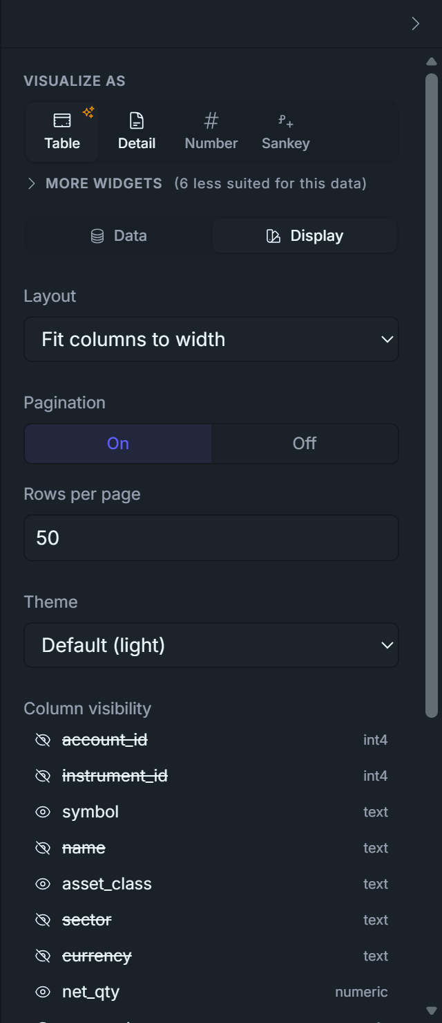
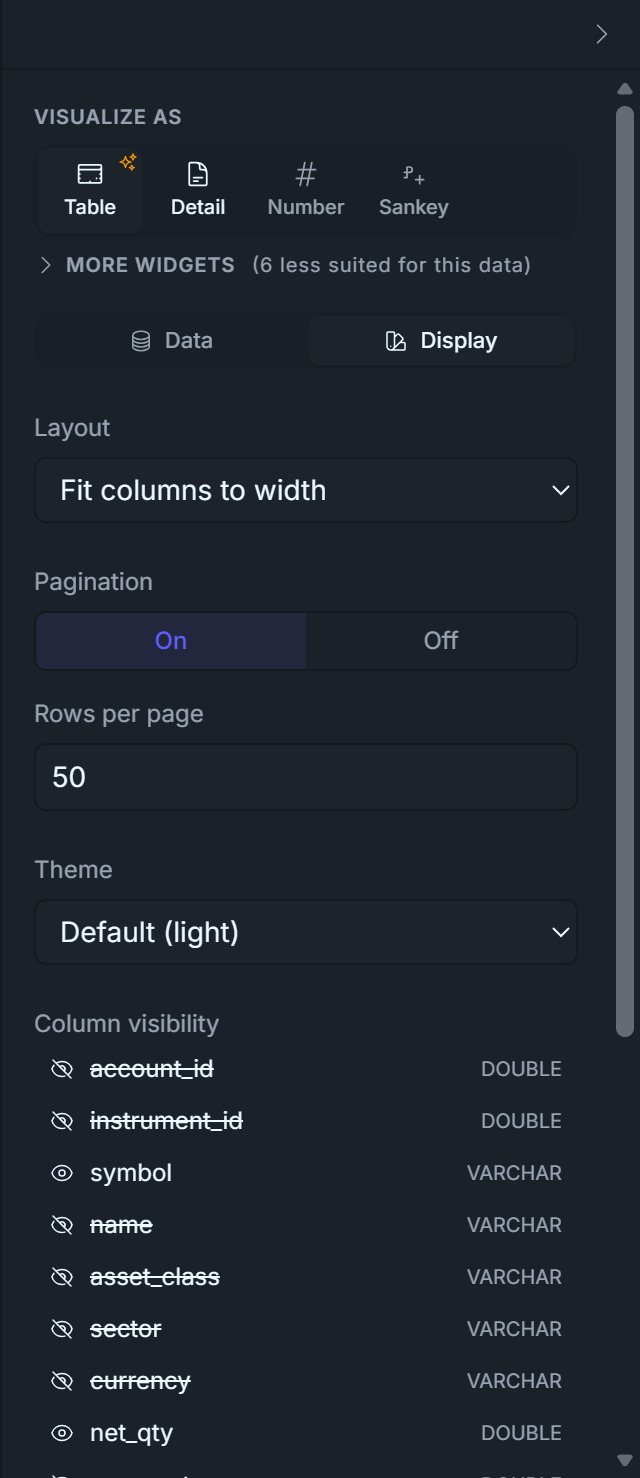
Open the right panel → Display tab. Toggle column visibility so only these are shown, in this order:
symbol — instrument ticker
asset_class — stock / etf / option / etc.
net_qty — signed; positive = long, negative = short
avg_cost — VWAP of the position's fills
mark_price — last available price from bar_1m
unrealized_pnl — (mark - cost) × net_qty, signed
pct_of_portfolio — |net_value| / account_equity
Add a Text Block above the table. Drop a UI Element → Text Block, type Current Positions. Resize to a thin header row. (You could also use the Tabulator's own Title field — that puts the title inside the widget frame. The Text Block approach gives more layout control.)
That's it. No SQL, no joins from the widget's perspective — the visual builder reads v_positions_marked like any other table.
Sanity check on the math. Look at any row with negative net_qty (a short). If mark_price < avg_cost, unrealized_pnl should be positive — that's a winning short. The view's (mark - cost) × net_qty handles long and short uniformly because both signs flip together.
Display tab — toggle OFF these columns (the rest stay on):
account_id, instrument_id (bookkeeping IDs)
name, sector, currency (duplicate / not useful)
mark_ts (timestamp clutter)
unrealized_pnl_pct, net_value, gross_value (covered by other widgets on this dashboard)
account_equity, account_max_leverage (constant across rows)
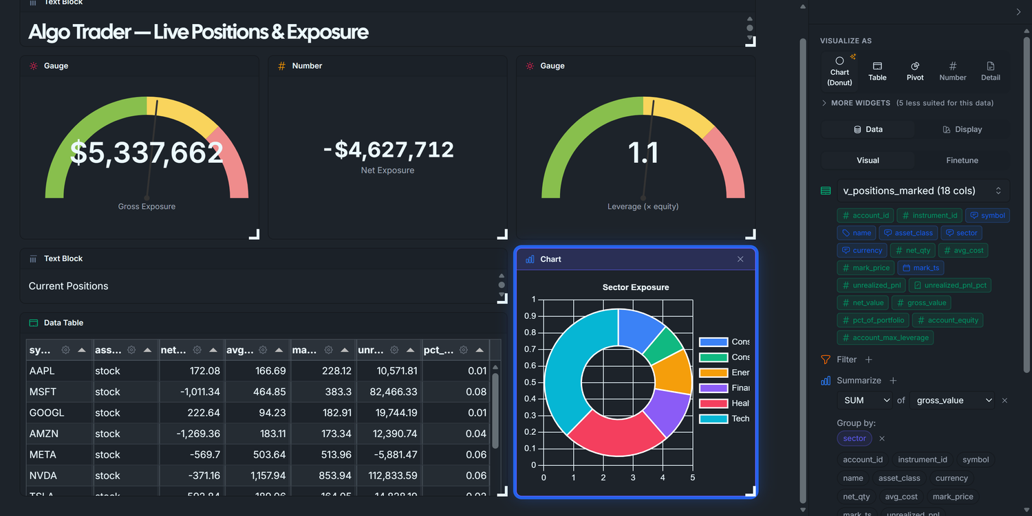
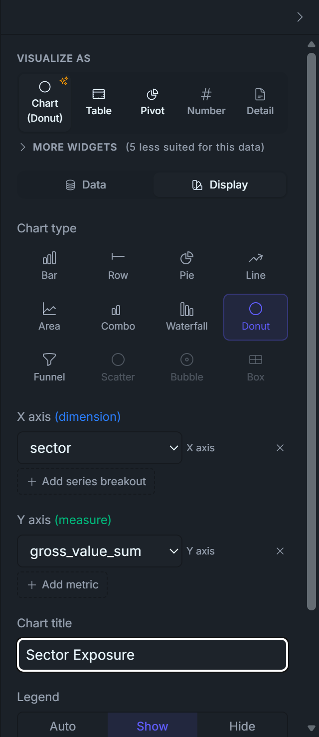
Phase 5 — Widget 5: Sector Donut
The "where is my money?" picture: one slice per sector, sized by total gross exposure.
Drag v_positions_marked onto the canvas (drop it next to the Current Positions table).
Data tab → Group by + → sector.
Summarize + → SUM of gross_value.
Run Query — you should get ~6 rows: Technology, Consumer Discretionary, Healthcare, Energy, Financials, Consumer Staples.
Display tab → Chart type → Doughnut(Donut in some menus). Legend → Show.
That's it. The auto-promote logic populates labelField: sector and datasets[0].field: gross_value_sum from your visual query; the doughnut renderer takes it from there.
Doughnut vs. Pie? Same data, different center. Doughnut leaves a hole that you can layer with a Total widget if you want; Pie is denser. Pure preference — both render correctly here.
Display tab — set:
Visualize As: Chart
Chart Type: Doughnut
Legend: Show
Title: Sector Exposure
Phase 6 — Widgets 6 & 7: Top 5 Winners & Losers
The "best and worst positions right now" pair. Both widgets target v_positions_marked, both show the same four columns; only the ORDER BY direction differs.
6.1 — Top 5 Winners
Drag v_positions_marked onto the canvas. A Data Table appears.
Data tab → Sort + → column unrealized_pnl, direction DESC.
Limit: change 500 → 5.
Display tab → toggle column visibility — leave only these four visible:
symbol
net_qty
unrealized_pnl
unrealized_pnl_pct
Hide every other column. The four visible ones tell the whole story: which name, how big a position, how much it's up in dollars, how much it's up in percent.
Drop a UI Element → Text Block above the table, type Top 5 Winners.
Display tab — toggle OFF these columns (keeps symbol, net_qty, unrealized_pnl, unrealized_pnl_pct):
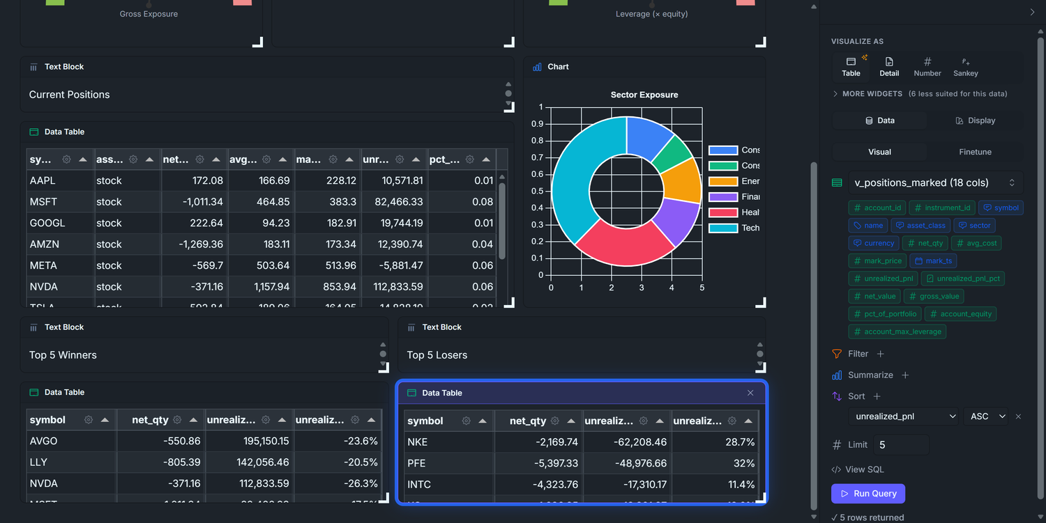
Identical to 5.1 with one change: Sort unrealized_pnl ASC — the most negative P&L sits at the top. Same four visible columns. Header text block: Top 5 Losers.
Place the two tables side-by-side under the Current Positions table.
Sanity check. A short position that has gone against you (mark > avg_cost on a net_qty < 0 row) shows unrealized_pnl < 0 because (mark - cost) × negative_qty < 0. So a moving-up market lands shorts in the losers table — which is correct. The view's signed math handles long and short uniformly.
Display tab — toggle OFF the same columns as the Winners table (keeps symbol, net_qty, unrealized_pnl, unrealized_pnl_pct):
Drag the widgets and arrange them as you wish. Below you have one possible example.
Two dashboards in the bag — and notice how much faster the second one came together once you'd seen the rhythm of drag → configure → publish on D1.
Stretch your legs, top up the coffee, then let's knock out the third one.
Dashboard 3 — Execution Quality
The am I getting filled at the prices I expect? dashboard — the one that catches a broken algo before P&L does. Most teams skip this for months and regret it.
D1 (P&L) tells you that something is wrong, days late. This dashboard tells you what and why, in real time (almost). Watch this during market hours — it's how you spot bad fills, latency spikes, and rejection storms before they show up on the P&L curve.
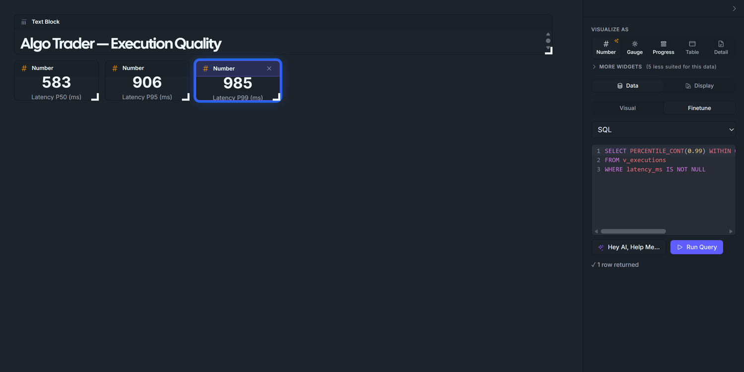
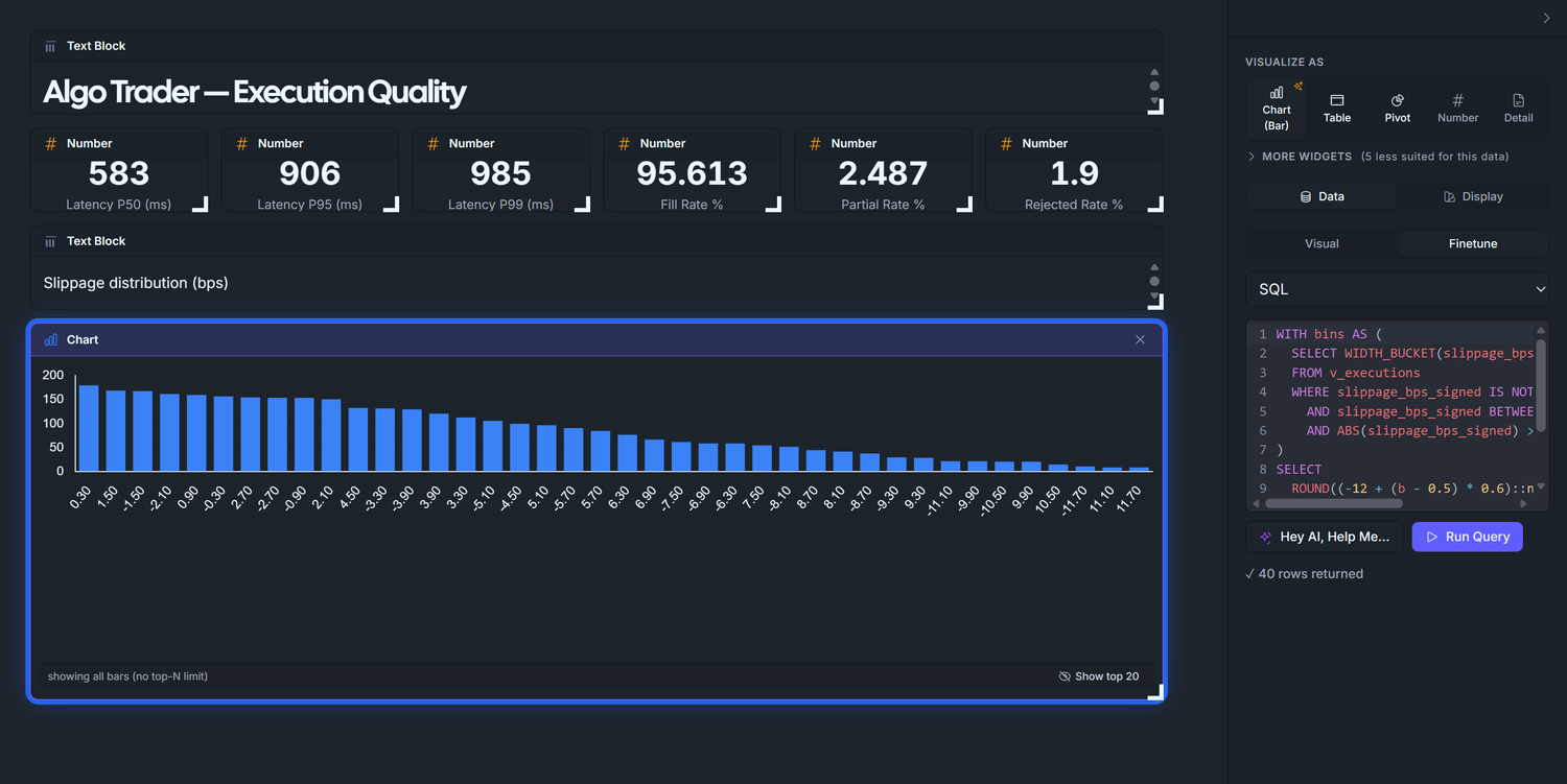
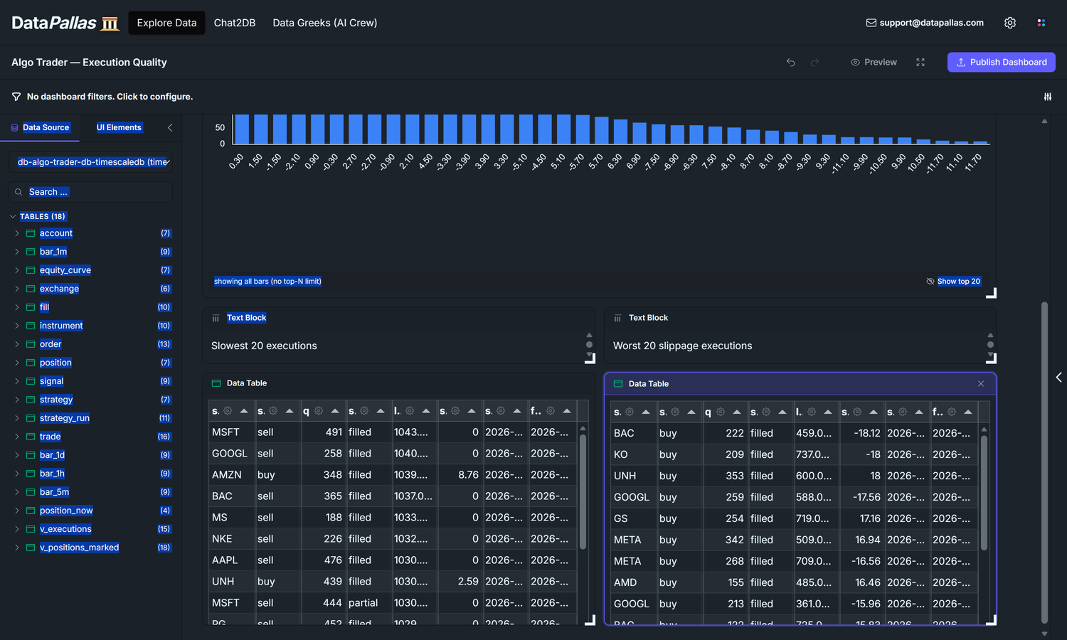
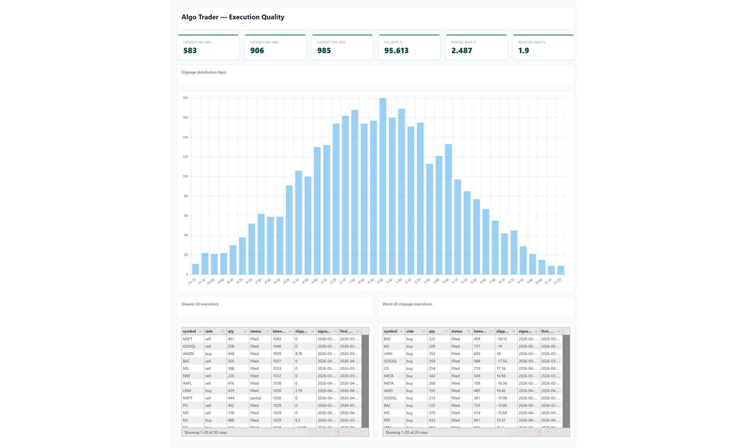
Our goal is to end up with a dashboard that looks roughly like this — six KPI tiles across the top (Latency P50 / P95 / P99 in milliseconds, plus Fill / Partial / Rejected rate percentages), a full-width Slippage Distribution histogram, then Slowest 20 and Worst 20 slippage drill-down tables side-by-side:
The enemies this dashboard hunts. Four invisible forces quietly cut your P&L, and the only way to catch them is to watch the execution layer continuously:
Latency — every millisecond between "the algo decides to trade" and "the order is filled" is a millisecond the market price drifts away from what your model assumed. On a fast-moving instrument, a 200 ms slowdown can cost you a basis point of price per trade — forever.
Slippage — even with zero latency, you rarely get the exact price you wanted: the spread widens, the order book thins, your size pushes through multiple levels. Death by a thousand small cuts.
Partial fills — your algo asks for 100 shares and gets 60. You're now under-positioned in the direction you wanted, the remaining 40 sit unfilled, and the next price tick rewards/punishes you for a position you didn't intend.
Rejections — the broker refuses your order (wrong lot size, insufficient margin, halted symbol, risk-limit breach). Every rejection is a trade the strategy wanted to make and couldn't — a silent missed-P&L that nothing else in your stack will surface.
D1 records the damage after it's compounded into the equity curve. This dashboard catches each of these at the moment of impact, while you can still act.
Eight widgets:
Latency tiles — three Number widgets measuring how long it takes between the moment your algo emits a signal and the moment the order's first fill lands back in the database (literally the timestamp on the fill row minus the timestamp on the signal row, for the first fill of each order). The three numbers are statistical percentiles: P50 is the typical case (the median — half your orders are faster than this, half are slower), P95 catches the slow tail (95% of orders are at or below this), P99 catches the worst case short of extreme outliers. Why look at paper trading specifically? Because paper trading skips the real broker round-trip — the latency you see there is purely your own code's processing time. Anything above a few hundred ms means your code path is doing too much work, and it'll bleed even more once you wire a live broker in.
Outcome rate tiles — three Number widgets: Fill Rate, Partial Fill Rate, Rejected Order Rate. Together they answer "is the broker actually executing what I'm sending?"
Slippage histogram — distribution of execution slippage in basis points, signed by side so positive = bad regardless of buy/sell.
Worst latency and Worst slippage drill-down tables — the actual outlier orders behind the percentiles, ordered worst-first.
Phase 1 — Define v_executions(the seed script already created this view for you — nothing to run here, just read through so you understand what every D3 widget binds to)
The base view. Same pattern as Dashboard 2's view — one denormalised view, then point-and-click for every widget. Joins order × signal × first fill, reading signal.implied_price (populated by the seed at signal time, against the bar close that triggered the signal).
CREATE OR REPLACE VIEW v_executions ASWITH first_fill AS ( SELECT DISTINCT ON (order_id) order_id, ts AS first_fill_ts, price AS first_fill_price, qty AS first_fill_qty FROM fill ORDER BY order_id, ts)SELECT o.id AS order_id, o.strategy_run_id, o.signal_id, o.instrument_id, i.symbol, o.side, o.qty AS qty_submitted, o.status, s.ts AS signal_ts, o.ts_submitted, ff.first_fill_ts, ff.first_fill_price, s.implied_price, -- latency = signal → first fill, in milliseconds EXTRACT(EPOCH FROM (ff.first_fill_ts - s.ts)) * 1000 AS latency_ms, -- slippage in basis points, signed so positive = bad regardless of side CASE WHEN s.implied_price IS NULL OR s.implied_price = 0 THEN NULL WHEN o.side = 'buy' THEN (ff.first_fill_price - s.implied_price) / s.implied_price * 10000 ELSE (s.implied_price - ff.first_fill_price) / s.implied_price * 10000 END AS slippage_bps_signedFROM "order" oJOIN signal s ON s.id = o.signal_idJOIN instrument i ON i.id = o.instrument_idLEFT JOIN first_fill ff ON ff.order_id = o.id;
Design notes:
DISTINCT ON (order_id) … ORDER BY ts picks the FIRST fill per order — the right reference for latency. (The seed writes one fill per order; the view is forward-compatible with multi-fill orders.)
Signed slippage: a buy filled above the implied price is bad (paid more); a sell filled below is also bad (got less). The CASE flips the sign so a single histogram of slippage_bps_signed shows positive = bad regardless of direction. Without the flip, sells would mirror-image the buys and the distribution would look symmetric and meaningless.
signal.implied_price is populated at signal-emit time in the seed (the bar close that triggered the signal). No downstream JOIN needed for the implied price — the view is a flat read.
LEFT JOIN the fill: orders that never filled (rejected) still appear, with latency_ms and slippage_bps_signed as NULL — useful for the drill-down tables.
The seed already creates this view alongside v_positions_marked (Appendix B), so a clean install gets it automatically. Pasting the DDL above into the Seed Data tab is only useful if you re-shape the view; the canvas tables panel surfaces v_executions next to the tables (DataPallas surfaces views and tables together because the schema-fetcher requests both TABLE and VIEW types from JDBC).
Naming. Same v_ prefix convention as v_positions_marked — dashboard helper view, not core schema.
Phase 2 — Title block
Set up a fresh canvas for this dashboard and drop a heading text block at the top before any data widget. Same flow as the previous two dashboards — see Dashboard 1 Phase 1 if you need the full step-by-step.
Explore Data → Create new canvas → rename to Algo Trader — Execution Quality.
Pick your TimescaleDB connection from the Data Source dropdown. The schema browser populates with v_executions alongside the base tables.
Click the UI Elements tab → drag a Text Block widget onto the canvas at the top.
With the text block selected, type into the right panel's Text input:
# Algo Trader — Execution Quality
Click the Data Source tab to switch back. Ready to add data widgets.
Phase 3 — Latency KPI tiles (P50 / P95 / P99)
Three Number widgets across the top. Percentiles need Finetune SQL — PERCENTILE_CONT can't be expressed via the Summarize UI (it isn't a single-column aggregation; it's a within-group construct).
DataPallas mode switch. Every widget in this phase uses Display tab → Finetune → SQL. The default Visual mode can't express PERCENTILE_CONT or COUNT(*) FILTER (WHERE …). If you ever see "no aggregation yet" in the canvas, you're in Visual mode — flip to Finetune → SQL.
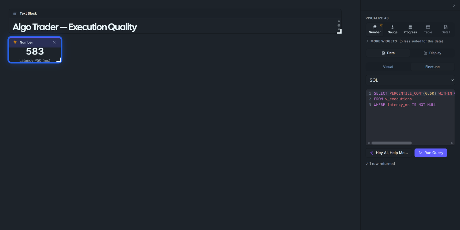
3.1 — P50 latency
Drag v_executions from the left panel onto the canvas (top-left).
Right panel → Visualize as → Number.
Right panel → Display → Finetune → SQL. Paste:
SELECT PERCENTILE_CONT(0.50) WITHIN GROUP (ORDER BY latency_ms) AS p50_msFROM v_executionsWHERE latency_ms IS NOT NULL
Run Query → single number around 400-600 ms (the seed simulates 150-1050 ms signal-to-fill latency, median in the middle).
Chart title: Latency P50 (ms) — set via the Number widget's Label field.
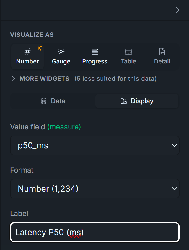
Display tab — set:
Visualize As: Number
Label: Latency P50 (ms)
Format: leave as default Number
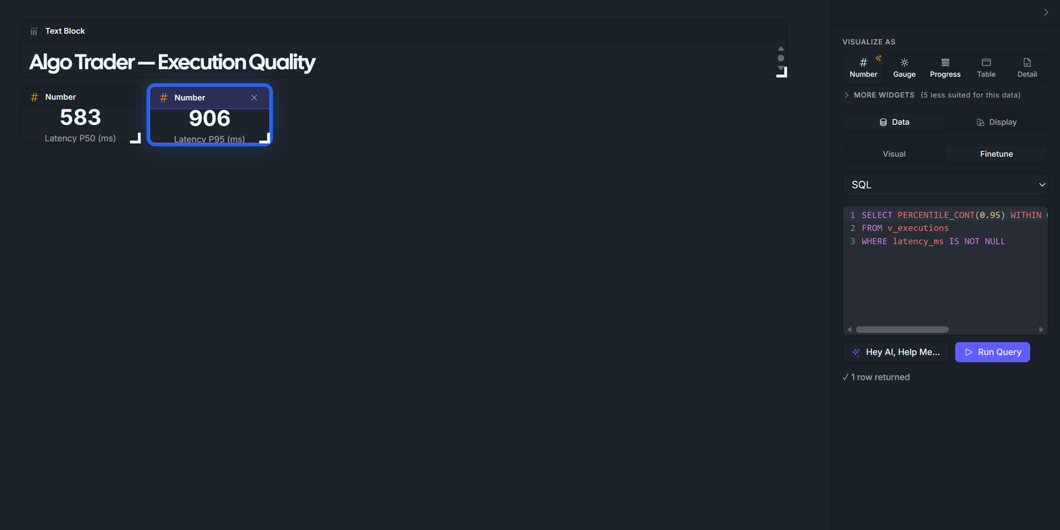
3.2 — P95 latency
Duplicate the P50 widget, change the percentile to 0.95, retitle to Latency P95 (ms). Expected ~900 ms for the seed. In production, P95 is the alarm bell: a sudden jump from 200ms to 2,000ms means a network or broker-side issue.
Display tab — set:
Visualize As: Number
Label: Latency P95 (ms)
Format: leave as default Number
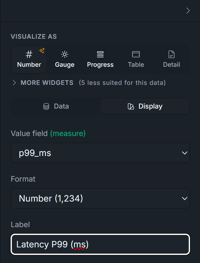
3.3 — P99 latency
Duplicate again, change to 0.99, retitle to Latency P99 (ms). Expected ~1000 ms. P99 is the "worst typical day" reading. Anything above ~5× P50 in production means the algo is occasionally hitting a slow path you should investigate.
Display tab — set:
Visualize As: Number
Label: Latency P99 (ms)
Format: leave as default Number
Why three tiles and not a single distribution chart? Operators read these in real time. A glanceable "P95 is 850ms today" is faster than parsing a histogram. The histogram in Phase 3 covers slippage, which doesn't have a single-number alarm threshold — but latency does, so the percentile tiles match the cognitive workflow.
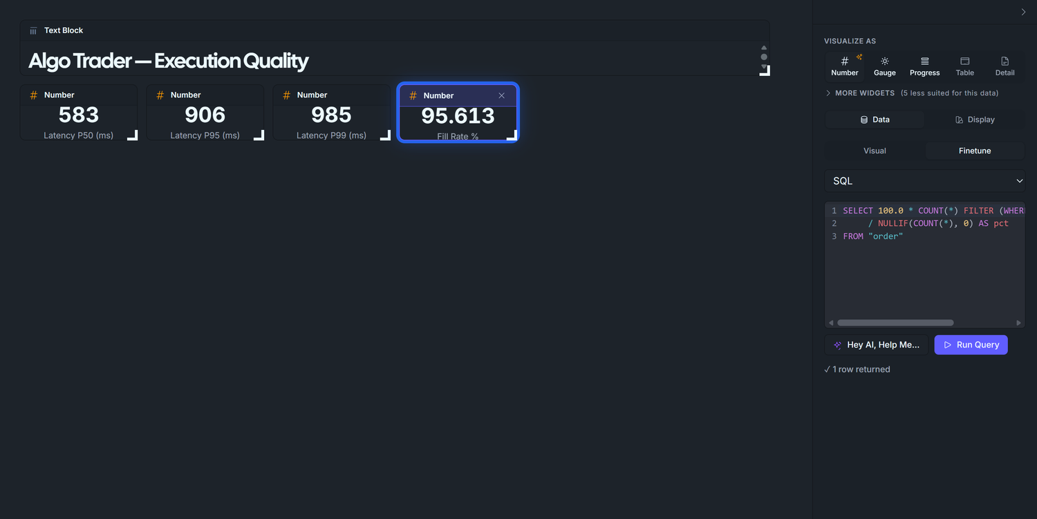
3.4 — Fill Rate
The "did the broker actually execute" KPI. Conditional aggregation — also needs Finetune → SQL.
Drag v_executions onto the canvas next to the latency tiles. Visualize as → Number.
Finetune → SQL:
SELECT 100.0 * COUNT(*) FILTER (WHERE status = 'filled') / NULLIF(COUNT(*), 0) AS pctFROM "order"
Run Query → ~95.2 (the seed targets 95%).
Chart title: Fill Rate %. The SQL multiplies by 100, so the displayed number 95.244 reads naturally as a percentage; no Format conversion needed.
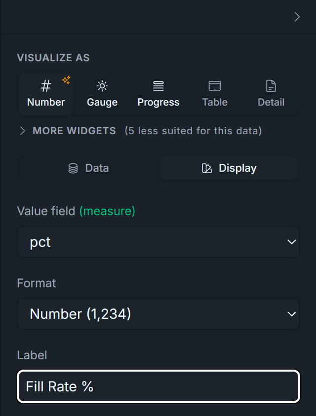
Display tab — set:
Visualize As: Number
Label: Fill Rate %
Format: leave as default Number (SQL pre-multiplies by 100 — 95.24 renders correctly without Percent format)
3.5 — Partial Fill Rate
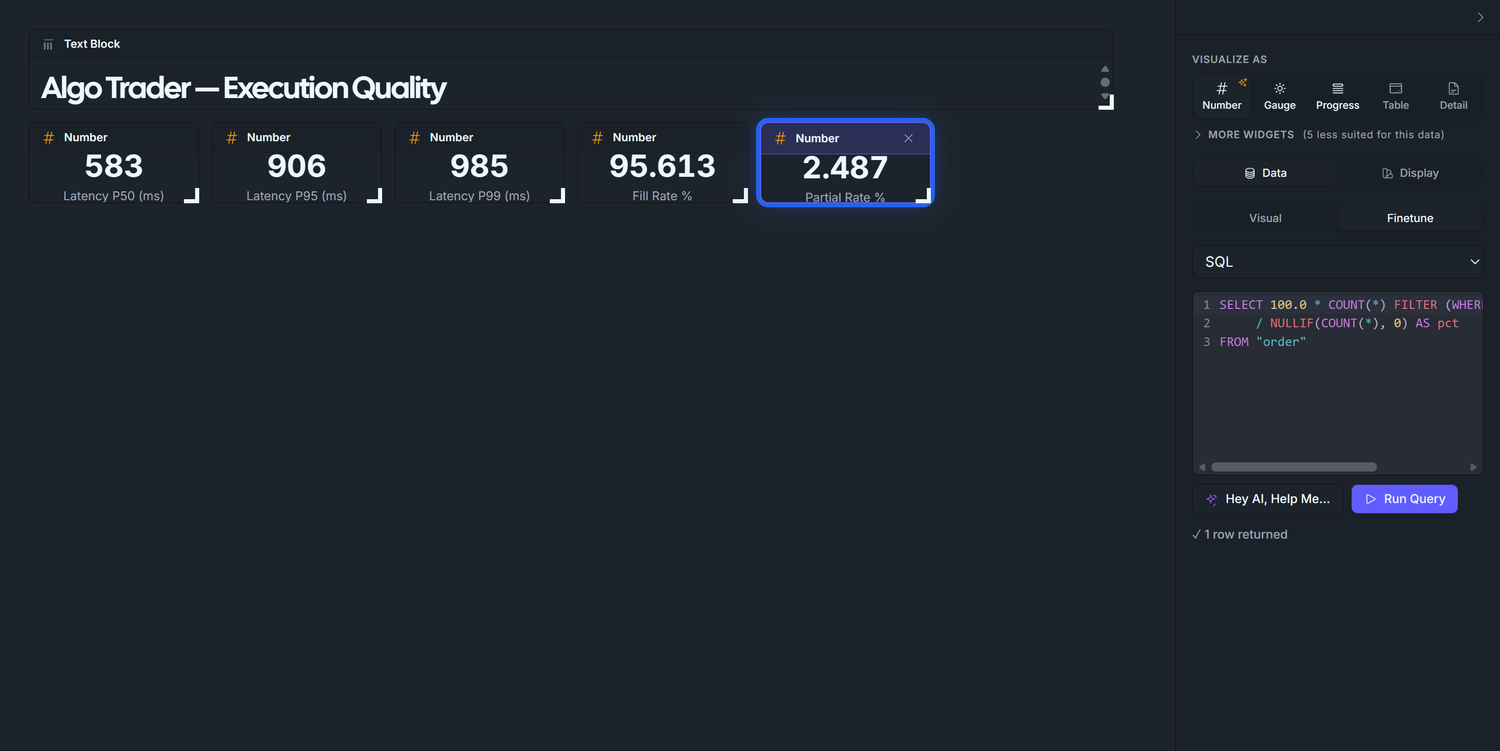
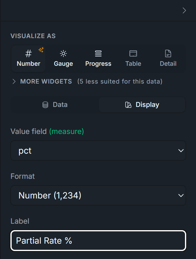
Duplicate 2.4, change WHERE status = 'filled' to WHERE status = 'partial', retitle to Partial Rate %. Expected ~2.9%. In production, a sustained partial-fill rate over ~5% means your order sizes are too aggressive for the venue's depth — split them.
Display tab — set:
Visualize As: Number
Label: Partial Rate %
Format: leave as default Number
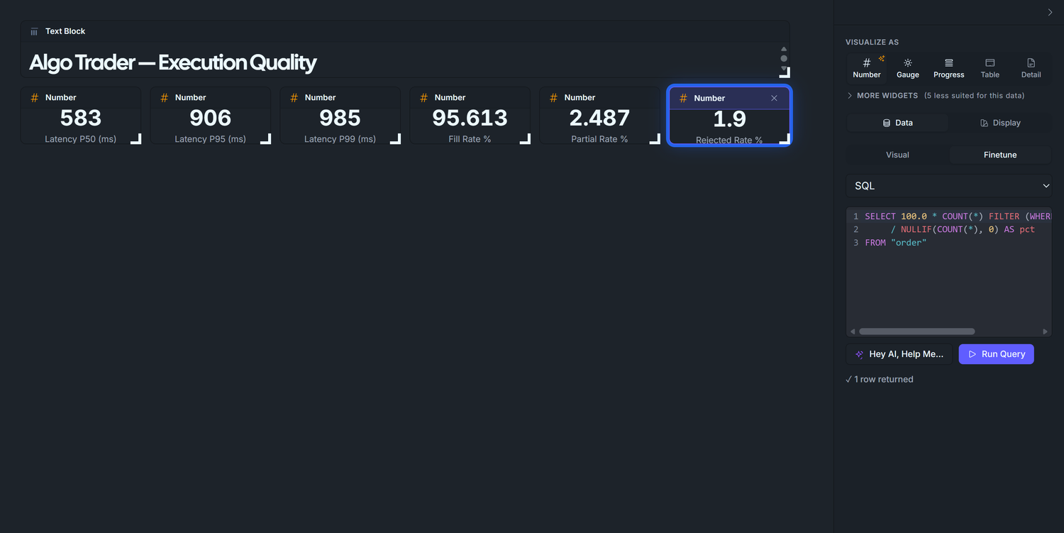
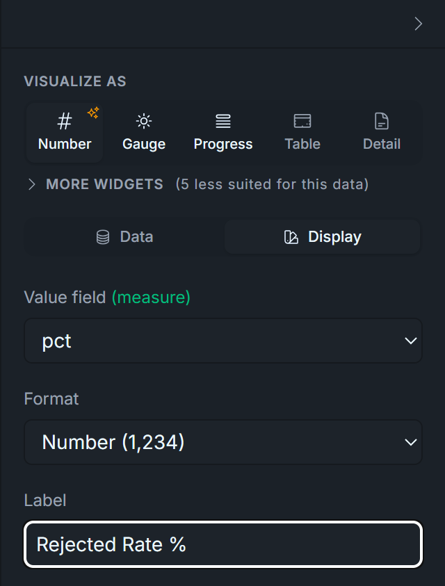
3.6 — Rejected Order Rate
Duplicate again, change to WHERE status = 'rejected', retitle to Rejected Rate %. Expected ~1.9%. Any spike here is the first place to look when P&L diverges suddenly: either a risk-layer config change just took effect, or the broker is throttling you.
Display tab — set:
Visualize As: Number
Label: Rejected Rate %
Format: leave as default Number
Why these three, not just one Fill Rate tile? Together they sum to 100% and give you the full lifecycle of a submitted order. A 95% Fill Rate alone hides whether the missing 5% is "broker rejected my orders outright" (alarming) or "I'm getting partials I should investigate" (operational). Three tiles make the failure mode obvious.
Phase 4 — Slippage histogram
A bar chart of slippage_bps_signed bucketed by WIDTH_BUCKET. We use Finetune → SQL (not the visual builder) for two reasons: (1) numerically-ordered x-axis behaviour is predictable, and (2) we need to filter out the synthetic zero-slippage rows the seed produces in the EOD-force-close and live-entry branches.
Seed gotcha — and the workaround. Roughly 50% of the rows in v_executions have slippage_bps_signed = 0 exactly: those are the EOD force-close and live-entry fills the seed writes without Gaussian noise. They aren't realistic executions; they're bookkeeping fills. Including them collapses the histogram into a single 4,000-tall spike at zero. The fix below filters them with ABS(slippage_bps_signed) > 0.001. (If you patch the seed to add * (1.0d + rand.nextGaussian() * 0.0005d) to those branches, the filter is no longer needed.)
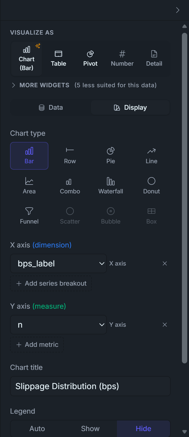
Drag v_executions onto the canvas (full-width row beneath the latency tiles). Visualize as → Bar.
Finetune → SQL:
WITH bins AS ( SELECT WIDTH_BUCKET(slippage_bps_signed, -12, 12, 40) AS b FROM v_executions WHERE slippage_bps_signed IS NOT NULL AND slippage_bps_signed BETWEEN -12 AND 12 AND ABS(slippage_bps_signed) > 0.001 -- excludes synthetic zero-slippage rows)SELECT b AS bucket_idx, ROUND((-12 + (b - 0.5) * 0.6)::numeric, 2)::text AS bps_label, COUNT(*) AS nFROM binsGROUP BY bORDER BY b
Run Query → ~40 rows, ascending by bucket_idx.
Right panel X axis (dimension): bps_label. Y axis (measure): n. Remove any extra metric the panel auto-added.
Chart title: Slippage distribution (bps). Legend: Hide.
Customize with DSL (Chart) — paste this minimal block:
chart { type 'bar' data { labelField 'bps_label' datasets { dataset { field 'n' label 'n' } } } options { plugins { legend { display false } } }}
This DSL is load-bearing: without it the bar chart sorts bins by count (so the shape reads as a downward slope), with it the chart respects the SQL's ORDER BY b and the distribution renders as a bell.
What you should see: a clean bell centred on 0 bps, peak ~170 in the middle bins, tails out to ~10 at ±11 bps. What to look for in production:
Fat right tail = your algo is chasing — sending market orders into thin books, or arriving late and paying up. Tighten limit orders or slow down the fire-rate.
Bimodal distribution = two distinct execution paths (e.g. one venue has stale quotes). Check fill.venue partitioning.
Centre shifted off zero = systematic adverse selection. Re-examine signal timing.
Why ±12 bps with 40 buckets? A diagnostic SELECT MIN, MAX, STDDEV, PERCENTILE_CONT(0.01), PERCENTILE_CONT(0.99) FROM v_executions on this seed returns stddev ≈ 3.6 bps, p01/p99 ≈ ±10.5. ±12 captures 99%+ of real noise; 40 buckets (0.6 bps wide each) gives ~25 visible bars across the bell. If your real broker has tighter or wider noise, re-run that diagnostic and re-bucket.
Display tab — set:
Visualize As: Chart
Chart Type: Bar
X axis: bps_label
Y axis: n
Title: Slippage Distribution (bps)
Legend: Hide
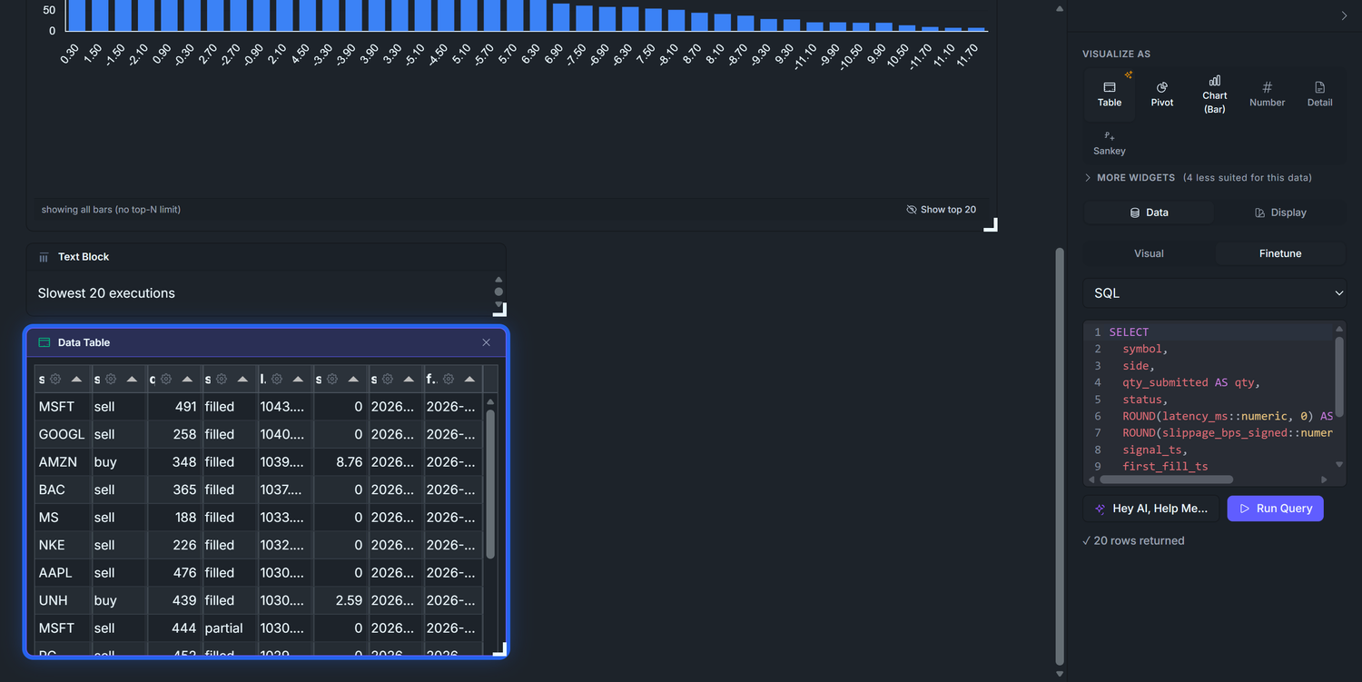
Phase 5 — Drill-down: worst 20 orders
Two tables side-by-side. Same view, different ORDER BY — exact same pattern as D2's Top Winners / Losers.
5.1 — Slowest 20 executions
Drag v_executions onto the canvas. Visualize as → Table.
Finetune → SQL:
SELECT symbol, side, qty_submitted AS qty, status, ROUND(latency_ms::numeric, 0) AS latency_ms, ROUND(slippage_bps_signed::numeric, 2) AS slippage_bps, signal_ts, first_fill_tsFROM v_executionsWHERE latency_ms IS NOT NULLORDER BY latency_ms DESCLIMIT 20
Chart title: Slowest 20 executions — set via a Text Block above the table (same pattern as D2's Top 5 Winners/Losers; there's no per-Tabulator Title input in the config UI).
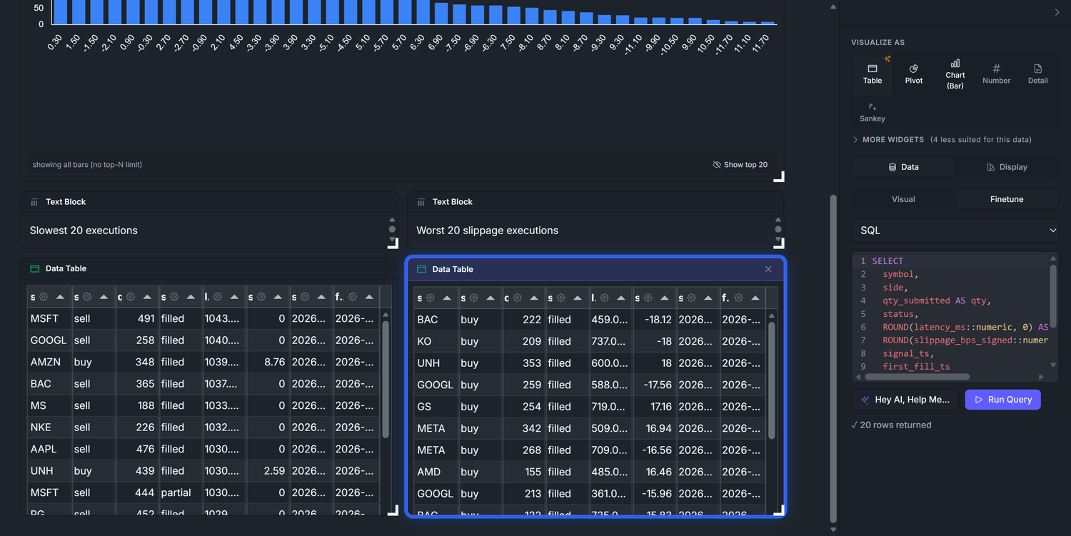
5.2 — Worst 20 slippage executions
Drag v_executions again. Visualize as → Table. SQL:
SELECT symbol, side, qty_submitted AS qty, status, ROUND(latency_ms::numeric, 0) AS latency_ms, ROUND(slippage_bps_signed::numeric, 2) AS slippage_bps, signal_ts, first_fill_tsFROM v_executionsWHERE slippage_bps_signed IS NOT NULLORDER BY ABS(slippage_bps_signed) DESCLIMIT 20
Title: Worst 20 slippage executions — same Text Block-above-table pattern as 5.1. The ABS(...) ordering is the key trick: most-positive-or-most-negative bubbles up, regardless of buy/sell direction.
Why two tables with identical column lists? They're scanned by different operators with different mental models. The latency table is read by infra/SRE: "show me the slow ones, did the network hiccup?" The slippage table is read by the strategy author: "show me the painful fills, was my signal early or late?" Same data, different lens — and side-by-side puts both lenses in front of one human at once.
These two tables are where the dashboard earns its keep. Click into a high-latency row → ask "why was this order slow?" → does it correlate with a specific instrument? Time of day? You'll spot the systemic issue from a handful of outliers, not from the percentile tile.
Phase 6 — Final layout
Drag the eight widgets into the layout below using the canvas's grid handles. No filter bar in v1 — the dashboard is a "show me everything that happened" view; if you need to scope by run or time window, add the same Strategy Runs filter D1 has (Phase 5 of D1) and bind it to each widget's SQL with WHERE strategy_run_id IN (${strategy_runs}) AND signal_ts BETWEEN ${from} AND ${to}.
Click Publish Dashboard
If you build only one operational dashboard, build this one.
And that's three. Does it work?, what am I holding right now?, am I getting filled at the prices I expect? — every question an algo trader needs answered every day, each now sitting on its own URL you can bookmark, share, or embed.
That's the mandatory set. Pour yourself a longer coffee this time — you earned it. The two bonus dashboards below are sketches and specs, not full walkthroughs, so feel free to pick them up whenever.
Bonus dashboards (sketches only)
Two more dashboards round out the trader's toolkit. We're not walking through them step-by-step — by now you've built three, and the Hey AI, Help Me… button has your back for anything you get stuck on. Instead, this section gives you exactly what you need to build each one yourself: the question it answers, the widget list with grid positions, the SQL each widget runs, and the chart / axis bindings.
Dashboard 4 — Trade Journal
The what's actually happening inside my trades? dashboard — the per-round-trip view that turns aggregate P&L into a shape you can read. Trades land in the trade table only after they close (a closing fill completes the round-trip), so this is end-of-day review, not live monitoring.
Filter — Strategy Runs (above the canvas grid). Same multiselect parameter as D1 (strategy_runs, default *). Every widget's SQL ends with WHERE strategy_run_id IN (${strategy_runs}).
Row 1 — KPI tiles (six Number widgets, each w=2 h=1):
#
Title
SQL
Format
1
Round-Trips
SELECT COUNT(*) FROM trade WHERE strategy_run_id IN (${strategy_runs})
Number (integer)
2
Avg Win $
SELECT AVG(net_pnl) FROM trade WHERE net_pnl > 0 AND strategy_run_id IN (${strategy_runs})
Currency
3
Avg Loss $
SELECT AVG(net_pnl) FROM trade WHERE net_pnl < 0 AND strategy_run_id IN (${strategy_runs})
Currency
4
Avg Hold (min)
SELECT AVG(holding_period_minutes) FROM trade WHERE strategy_run_id IN (${strategy_runs})
Number (1 decimal)
5
Win / Loss Ratio
SELECT AVG(net_pnl) FILTER (WHERE net_pnl > 0) / NULLIF(-AVG(net_pnl) FILTER (WHERE net_pnl < 0), 0) FROM trade WHERE strategy_run_id IN (${strategy_runs})
Number (2 decimals)
6
% Profitable
SELECT 100.0 * COUNT(*) FILTER (WHERE net_pnl > 0) / NULLIF(COUNT(*), 0) FROM trade WHERE strategy_run_id IN (${strategy_runs})
Percent
Row 2 — P&L per round-trip histogram (Chart, Bar, w=12 h=4). Add a Text Block header above ("P&L per round-trip ($)"):
WITH bins AS ( SELECT WIDTH_BUCKET(net_pnl, -500, 500, 40) AS b FROM trade WHERE strategy_run_id IN (${strategy_runs}) AND net_pnl BETWEEN -500 AND 500)SELECT ROUND((-500 + (b - 0.5) * 25)::numeric, 0)::text AS pnl_bucket, COUNT(*) AS nFROM binsGROUP BY bORDER BY b
Chart Type: Bar. X axis: pnl_bucket. Y axis: n. Legend: hide. Apply the same minimal DSL pattern as D3's slippage histogram with labelField 'pnl_bucket' so the bins render in numeric order (the canvas-builder otherwise sorts bars by count desc and the shape is lost).
What to look for: a right-skewed long tail = letting winners run (good). Symmetric bell or left-skewed = cutting winners short / letting losers run. Widen the ±500 range if you see clipping at the edges.
Row 3 (left) — Holding-period histogram (Chart, Bar, w=6 h=4). Text Block header: "Holding period (minutes)":
WITH bins AS ( SELECT WIDTH_BUCKET(holding_period_minutes, 0, 240, 40) AS b FROM trade WHERE strategy_run_id IN (${strategy_runs}) AND holding_period_minutes BETWEEN 0 AND 240)SELECT ROUND((b - 0.5) * 6.0, 1)::text AS minutes_bucket, COUNT(*) AS nFROM binsGROUP BY bORDER BY b
X axis: minutes_bucket. Y axis: n. Same DSL labelField 'minutes_bucket' pattern.
What to look for: a single mode = one strategy. Bimodal = two strategies in one algo (e.g. scalp + swing) — split them out.
Row 3 (right) — MFE / MAE scatter (Chart, Scatter, w=6 h=4). Text Block header: "MFE / MAE scatter":
SELECT mfe AS mfe, ABS(mae) AS mae_abs, CASE WHEN net_pnl > 0 THEN 'win' ELSE 'loss' END AS outcomeFROM tradeWHERE strategy_run_id IN (${strategy_runs})
Chart Type: Scatter. X axis: mfe. Y axis: mae_abs. Group / colour by: outcome (so wins and losses get different colours).
What to look for: dots below the y = x diagonal = healthy (the trade ran further in your favour than against). Losers near the X-axis = took the loss early; losers far up and to the right = let losers run before cutting.
Dashboard 5 — Market Data Health
The is my market data complete and fresh? dashboard — the silent-disaster prevention layer. With the seed every minute is filled, so most cells will report a clean state; this dashboard is built for the moment your real ingestion pipeline starts dropping bars or stops updating.
No filter bar in v1. This dashboard reports the current state of the entire bar_1m hypertable across all instruments. If you need to scope to a date window later, wire a from / to parameter (same pattern as D1's Strategy Runs) and add WHERE ts BETWEEN ${from} AND ${to} to each widget's SQL.
Row 1 — KPI tiles (four Number widgets, each w=3 h=1):
#
Title
SQL
Format
1
Total bars
SELECT COUNT(*) FROM bar_1m
Number (integer)
2
Active instruments
SELECT COUNT(*) FROM instrument WHERE is_active
Number (integer)
3
Last bar age (min)
SELECT EXTRACT(EPOCH FROM (NOW() - MAX(ts))) / 60 FROM bar_1m
Number (1 decimal)
4
Days with gaps
(SQL below)
Number (integer)
Days-with-gaps SQL — count of (instrument, day) cells whose bar count is below the 390-bars-per-session expectation (US session = 9:30 → 16:00 ET = 390 minutes):
WITH day_counts AS ( SELECT instrument_id, DATE_TRUNC('day', ts) AS day, COUNT(*) AS bars_in_day FROM bar_1m GROUP BY instrument_id, DATE_TRUNC('day', ts))SELECT COUNT(*) FROM day_counts WHERE bars_in_day < 390
On a fresh seed this returns 0 — by design no gaps are generated. The widget exists so the moment your real ingest drops a bar this stops being 0.
Row 2 (left) — Bars per instrument (Chart, Bar, w=8 h=4). Text Block header: "Bars per instrument":
SELECT i.symbol AS symbol, COUNT(*) AS nFROM bar_1m bJOIN instrument i ON i.id = b.instrument_idGROUP BY i.symbolORDER BY n DESC
Chart Type: Bar. X axis: symbol. Y axis: n. Click Show all bars so all ~30 instruments render. Apply DSL labelField 'symbol' to preserve the SQL's DESC order (otherwise the canvas-builder sorts and limits the bars).
What to look for: a uniform horizon of similar-height bars = healthy. One bar visibly shorter = that instrument missed one or more session days. Several short bars together = ingestion outage.
SELECT i.symbol AS symbol, MAX(b.ts) AS last_bar_ts, EXTRACT(EPOCH FROM (NOW() - MAX(b.ts))) / 60 AS age_minutesFROM instrument iLEFT JOIN bar_1m b ON b.instrument_id = i.idGROUP BY i.symbolORDER BY age_minutes DESC NULLS FIRSTLIMIT 20
What to look for: during a live session age_minutes should be ≤ 2 for every active symbol. A symbol with NULLlast_bar_ts = an instrument with zero ingestion (LEFT JOIN surfaces them; NULLS FIRST floats them to the top).
Row 3 — Bar gaps — instrument × day (Tabulator, w=12 h=4). Text Block header: "Bar gaps — instrument × day (rows with bars_in_day < 390)":
WITH day_counts AS ( SELECT instrument_id, DATE_TRUNC('day', ts) AS day, COUNT(*) AS bars_in_day FROM bar_1m GROUP BY instrument_id, DATE_TRUNC('day', ts))SELECT i.symbol AS symbol, dc.day AS day, dc.bars_in_day AS bars_in_day, (390 - dc.bars_in_day) AS gap_countFROM day_counts dcJOIN instrument i ON i.id = dc.instrument_idWHERE dc.bars_in_day < 390ORDER BY (390 - dc.bars_in_day) DESC, dc.day DESCLIMIT 50
What to look for: on a clean day the query returns 0 rows. A single row = one missing minute on one instrument (usually ignorable). A cluster of rows on the same day across many symbols = vendor outage. A column of rows on the same symbol across consecutive days = that instrument's pipeline broke.
Going further
A short tour of where this design grows.
Crypto switch. Two tables touched, recapped from the Crypto adaptation note in 4 layers, 12 tables:
exchange — populate the existing code column ("binance", "coinbase") instead of mic (crypto venues have no MIC code). No schema change.
instrument — ALTER TABLE instrument ADD COLUMN quote_currency TEXT so BTC/USDT and BTC/USD are distinct rows; and drop lot_size enforcement at order-validation time (the column stays, the validator's integer-multiples check no longer applies). One new column, one behavioural shift.
Every dashboard, query, and form keeps working.
Tick-level upgrade. When bars aren't enough — usually for high-frequency strategies, transaction-cost analysis, or spread/microstructure work — you graduate to a quote(instrument_id, ts, bid, ask, bid_size, ask_size) table. At >1M rows per day per symbol, Postgres struggles even with Timescale. This is the moment to put quotes (and only quotes) on ClickHouse, also available as a DataPallas starter pack. Everything else stays on Postgres/Timescale.
Risk layer. Pre-trade checks belong in a stored function called by the order insert path: max position size, max order notional, instrument blacklist per strategy, daily loss limit per account. Reject by raising — never by silently mutating the order. The account.kill_switch boolean is the global override.
Backtest reproducibility.strategy_run.params_snapshot_json + market_data_window_hash is enough for "rerun this exact backtest tomorrow and get the same numbers." Add strategy.commit_sha if your algos live in git, and you can also reproduce the code.
Appendix — Files
Seed script (single Groovy file): paste into the Seed Data tab. Creates the 12 tables, hypertable, continuous aggregates, the position_now view, ~30 instruments, 90 days of bars, 4 strategies, 200 runs with full lifecycle data. Full source in Appendix B below — copy/paste ready.
Closing thought
A trading platform's value isn't in how many tables it has — it's in whether the four layers are honest about what's primary and what's derived. Bars are primary; aggregates are derived. Fills are primary; positions are derived. Signals are primary; trades are derived. Get that hierarchy right and your dashboards write themselves; get it wrong and you'll spend the next year reconciling tables that shouldn't have existed.
DataPallas gives you the rest — the database, the seeding, the dashboards, the connection management — for free. The only thing worth thinking hard about is the model. So think hard about the model.
Appendix B — Seed script source
Paste this into the Seed Data tab on your TimescaleDB connection and click Run. It creates the schema, generates synthetic market data, and simulates 200 strategy runs end-to-end. The script is idempotent — safe to re-run; existing tables are dropped and rebuilt.
// @description Algo Trader: 12-table data model + 90 days of intraday bars + 200 strategy runs//// Idempotent — safe to re-run. Every execution begins with DROP ... IF EXISTS CASCADE// for all 12 tables, the hypertable, the 3 continuous aggregates, and the position_now// view, in child-first order. Partial state from a failed previous run is wiped clean// before anything is recreated. Re-running after a successful run also works — same end// state, just slower.//// Bindings provided by GenericSeedExecutor:// dbSql — groovy.sql.Sql connected to the target database// vendor — String (uppercase): expects POSTGRES / POSTGRESQL / TIMESCALEDB / SUPABASE// log — SLF4J Logger// params — Map with optional keys: N_INSTRUMENTS (default 30), DAYS (default 90), N_RUNS (default 200)import net.datafaker.Fakerimport java.sql.Timestampimport java.time.*import java.time.temporal.ChronoUnitif (!(vendor in ['POSTGRES','POSTGRESQL','TIMESCALEDB','SUPABASE'])) { throw new RuntimeException("Algo Trader seeder requires PostgreSQL/TimescaleDB. Got: ${vendor}")}int N_INSTRUMENTS = params?.N_INSTRUMENTS ? Integer.parseInt(params.N_INSTRUMENTS.toString()) : 30int DAYS = params?.DAYS ? Integer.parseInt(params.DAYS.toString()) : 90int N_RUNS = params?.N_RUNS ? Integer.parseInt(params.N_RUNS.toString()) : 200long SEED = 42Lint BATCH_SIZE = 5000log.info("=== Algo Trader Seed: starting (instruments={}, days={}, runs={}) ===", N_INSTRUMENTS, DAYS, N_RUNS)def safe = { String s -> try { dbSql.execute(s) } catch (Exception e) { log.debug("DDL skipped: {}", e.message) } }// ── 1. Drop existing objects (child-first, idempotent) ───────────────────────safe("DROP MATERIALIZED VIEW IF EXISTS bar_1d CASCADE")safe("DROP MATERIALIZED VIEW IF EXISTS bar_1h CASCADE")safe("DROP MATERIALIZED VIEW IF EXISTS bar_5m CASCADE")safe("DROP VIEW IF EXISTS position_now CASCADE")safe("DROP TABLE IF EXISTS equity_curve CASCADE")safe("DROP TABLE IF EXISTS trade CASCADE")safe("DROP TABLE IF EXISTS position CASCADE")safe("DROP TABLE IF EXISTS fill CASCADE")safe('DROP TABLE IF EXISTS "order" CASCADE')safe("DROP TABLE IF EXISTS signal CASCADE")safe("DROP TABLE IF EXISTS strategy_run CASCADE")safe("DROP TABLE IF EXISTS bar_1m CASCADE")safe("DROP TABLE IF EXISTS strategy CASCADE")safe("DROP TABLE IF EXISTS account CASCADE")safe("DROP TABLE IF EXISTS instrument CASCADE")safe("DROP TABLE IF EXISTS exchange CASCADE")// ── 2. Schema: Layer 1 (reference) ───────────────────────────────────────────dbSql.execute("CREATE EXTENSION IF NOT EXISTS timescaledb")dbSql.execute(""" CREATE TABLE exchange ( id SERIAL PRIMARY KEY, code TEXT NOT NULL UNIQUE, mic TEXT, name TEXT NOT NULL, timezone TEXT NOT NULL, currency TEXT NOT NULL )""")dbSql.execute(""" CREATE TABLE instrument ( id SERIAL PRIMARY KEY, exchange_id INT NOT NULL REFERENCES exchange(id), symbol TEXT NOT NULL, asset_class TEXT NOT NULL, name TEXT, sector TEXT, currency TEXT NOT NULL, tick_size NUMERIC(10,4) DEFAULT 0.01, lot_size INT DEFAULT 1, is_active BOOLEAN DEFAULT TRUE, UNIQUE(exchange_id, symbol) )""")dbSql.execute(""" CREATE TABLE account ( id SERIAL PRIMARY KEY, broker TEXT NOT NULL, base_currency TEXT NOT NULL, equity NUMERIC(18,2) NOT NULL, max_leverage NUMERIC(5,2) DEFAULT 1.0, kill_switch BOOLEAN DEFAULT FALSE, created_at TIMESTAMPTZ DEFAULT now() )""")dbSql.execute(""" CREATE TABLE strategy ( id SERIAL PRIMARY KEY, name TEXT NOT NULL UNIQUE, version TEXT NOT NULL, description TEXT, params_schema_json JSONB, status TEXT DEFAULT 'active', created_at TIMESTAMPTZ DEFAULT now() )""")// ── 3. Schema: Layer 2 (market data) ─────────────────────────────────────────dbSql.execute(""" CREATE TABLE bar_1m ( instrument_id INT NOT NULL REFERENCES instrument(id), ts TIMESTAMPTZ NOT NULL, open NUMERIC(18,4) NOT NULL, high NUMERIC(18,4) NOT NULL, low NUMERIC(18,4) NOT NULL, close NUMERIC(18,4) NOT NULL, volume BIGINT NOT NULL, vwap NUMERIC(18,4), trade_count INT, PRIMARY KEY (instrument_id, ts) )""")dbSql.execute("SELECT create_hypertable('bar_1m', 'ts', chunk_time_interval => INTERVAL '7 days')")// Three continuous aggregates (5m, 1h, 1d) — written out explicitly because Groovy SQL// treats GString interpolation as JDBC parameter binding, and you can't parameterize identifiers.dbSql.execute(""" CREATE MATERIALIZED VIEW bar_5m WITH (timescaledb.continuous) AS SELECT instrument_id, time_bucket('5 minutes', ts) AS ts, first(open, ts) AS open, max(high) AS high, min(low) AS low, last(close, ts) AS close, sum(volume) AS volume, sum(close * volume) / nullif(sum(volume), 0) AS vwap, sum(trade_count) AS trade_count FROM bar_1m GROUP BY 1, 2 WITH NO DATA""")dbSql.execute(""" CREATE MATERIALIZED VIEW bar_1h WITH (timescaledb.continuous) AS SELECT instrument_id, time_bucket('1 hour', ts) AS ts, first(open, ts) AS open, max(high) AS high, min(low) AS low, last(close, ts) AS close, sum(volume) AS volume, sum(close * volume) / nullif(sum(volume), 0) AS vwap, sum(trade_count) AS trade_count FROM bar_1m GROUP BY 1, 2 WITH NO DATA""")dbSql.execute(""" CREATE MATERIALIZED VIEW bar_1d WITH (timescaledb.continuous) AS SELECT instrument_id, time_bucket('1 day', ts) AS ts, first(open, ts) AS open, max(high) AS high, min(low) AS low, last(close, ts) AS close, sum(volume) AS volume, sum(close * volume) / nullif(sum(volume), 0) AS vwap, sum(trade_count) AS trade_count FROM bar_1m GROUP BY 1, 2 WITH NO DATA""")// ── 4. Schema: Layer 3 (trading lifecycle) ───────────────────────────────────dbSql.execute(""" CREATE TABLE strategy_run ( id SERIAL PRIMARY KEY, strategy_id INT NOT NULL REFERENCES strategy(id), account_id INT NOT NULL REFERENCES account(id), mode TEXT NOT NULL CHECK (mode IN ('backtest','paper','live')), from_ts TIMESTAMPTZ NOT NULL, to_ts TIMESTAMPTZ, params_snapshot_json JSONB, market_data_window_hash TEXT, status TEXT DEFAULT 'completed', started_at TIMESTAMPTZ DEFAULT now(), ended_at TIMESTAMPTZ )""")dbSql.execute(""" CREATE TABLE signal ( id BIGSERIAL PRIMARY KEY, strategy_run_id INT NOT NULL REFERENCES strategy_run(id), instrument_id INT NOT NULL REFERENCES instrument(id), ts TIMESTAMPTZ NOT NULL, side TEXT NOT NULL CHECK (side IN ('buy','sell','flat')), strength NUMERIC(5,4), reason_text TEXT, implied_price NUMERIC(18,4), source_bar_ts TIMESTAMPTZ )""")dbSql.execute(''' CREATE TABLE "order" ( id BIGSERIAL PRIMARY KEY, strategy_run_id INT NOT NULL REFERENCES strategy_run(id), signal_id BIGINT REFERENCES signal(id), instrument_id INT NOT NULL REFERENCES instrument(id), ts_submitted TIMESTAMPTZ NOT NULL, side TEXT NOT NULL, qty NUMERIC(18,4) NOT NULL, type TEXT NOT NULL CHECK (type IN ('market','limit','stop')), limit_price NUMERIC(18,4), time_in_force TEXT DEFAULT 'DAY', status TEXT NOT NULL, ts_terminal TIMESTAMPTZ, parent_order_id BIGINT )''')dbSql.execute(''' CREATE TABLE fill ( id BIGSERIAL PRIMARY KEY, order_id BIGINT NOT NULL REFERENCES "order"(id), ts TIMESTAMPTZ NOT NULL, qty NUMERIC(18,4) NOT NULL, qty_signed NUMERIC(18,4) NOT NULL, price NUMERIC(18,4) NOT NULL, fee NUMERIC(18,4) DEFAULT 0, venue TEXT, liquidity_flag TEXT CHECK (liquidity_flag IN ('maker','taker')), external_id TEXT )''')dbSql.execute(""" CREATE TABLE position ( account_id INT NOT NULL REFERENCES account(id), instrument_id INT NOT NULL REFERENCES instrument(id), ts TIMESTAMPTZ NOT NULL, qty NUMERIC(18,4) NOT NULL, avg_cost NUMERIC(18,4), realized_pnl NUMERIC(18,2), last_fill_id BIGINT, PRIMARY KEY (account_id, instrument_id, ts) )""")// position_now: derived view — one row per (account, instrument) currently holding a non-zero net qtydbSql.execute(''' CREATE VIEW position_now AS SELECT sr.account_id, o.instrument_id, sum(f.qty_signed) AS net_qty, sum(f.qty_signed * f.price) / nullif(sum(f.qty_signed), 0) AS avg_cost FROM fill f JOIN "order" o ON o.id = f.order_id JOIN strategy_run sr ON sr.id = o.strategy_run_id GROUP BY 1, 2 HAVING sum(f.qty_signed) <> 0''')// v_positions_marked: Dashboard 2's single base view — positions ⋈ latest bar ⋈ instrument ⋈ account.// Computes mark price, unrealized P&L (absolute + %), gross / net exposure, % of portfolio. Every// Dashboard 2 widget (positions table, gauges, top winners/losers, asset-class donut) reads from// this view via the visual builder — no per-widget joins needed.// Documented in the Dashboard 2 walkthrough above; same DDL repeated here so a clean install gets it.dbSql.execute(''' CREATE OR REPLACE VIEW v_positions_marked AS WITH latest_bar AS ( SELECT DISTINCT ON (instrument_id) instrument_id, ts AS mark_ts, close AS mark_price FROM bar_1m ORDER BY instrument_id, ts DESC ) SELECT pn.account_id, pn.instrument_id, i.symbol, i.name, i.asset_class, i.sector, i.currency, pn.net_qty, pn.avg_cost, lb.mark_price, lb.mark_ts, (lb.mark_price - pn.avg_cost) * pn.net_qty AS unrealized_pnl, CASE WHEN pn.avg_cost <> 0 THEN (lb.mark_price - pn.avg_cost) / pn.avg_cost ELSE NULL END AS unrealized_pnl_pct, pn.net_qty * lb.mark_price AS net_value, abs(pn.net_qty) * lb.mark_price AS gross_value, abs(pn.net_qty * lb.mark_price) / NULLIF(a.equity, 0) AS pct_of_portfolio, a.equity AS account_equity, a.max_leverage AS account_max_leverage FROM position_now pn JOIN latest_bar lb ON lb.instrument_id = pn.instrument_id JOIN instrument i ON i.id = pn.instrument_id JOIN account a ON a.id = pn.account_id''')// v_executions: Dashboard 3's single base view — order ⋈ signal ⋈ first fill ⋈ instrument.// Computes per-order latency (signal → first fill, in milliseconds) and signed slippage in// basis points (positive = bad regardless of buy/sell). All D3 widgets (latency percentile// tiles, fill-rate / partial / rejected tiles, slippage histogram, drill-down tables) read// from this view. Documented in the Dashboard 3 walkthrough; same DDL repeated here so a clean// install gets it.dbSql.execute(''' CREATE OR REPLACE VIEW v_executions AS WITH first_fill AS ( SELECT DISTINCT ON (order_id) order_id, ts AS first_fill_ts, price AS first_fill_price, qty AS first_fill_qty FROM fill ORDER BY order_id, ts ) SELECT o.id AS order_id, o.strategy_run_id, o.signal_id, o.instrument_id, i.symbol, o.side, o.qty AS qty_submitted, o.status, s.ts AS signal_ts, o.ts_submitted, ff.first_fill_ts, ff.first_fill_price, s.implied_price, EXTRACT(EPOCH FROM (ff.first_fill_ts - s.ts)) * 1000 AS latency_ms, CASE WHEN s.implied_price IS NULL OR s.implied_price = 0 THEN NULL WHEN o.side = 'buy' THEN (ff.first_fill_price - s.implied_price) / s.implied_price * 10000 ELSE (s.implied_price - ff.first_fill_price) / s.implied_price * 10000 END AS slippage_bps_signed FROM "order" o JOIN signal s ON s.id = o.signal_id JOIN instrument i ON i.id = o.instrument_id LEFT JOIN first_fill ff ON ff.order_id = o.id''')// ── 5. Schema: Layer 4 (analytics) ───────────────────────────────────────────dbSql.execute(""" CREATE TABLE trade ( id BIGSERIAL PRIMARY KEY, strategy_run_id INT NOT NULL REFERENCES strategy_run(id), instrument_id INT NOT NULL REFERENCES instrument(id), opened_at TIMESTAMPTZ NOT NULL, closed_at TIMESTAMPTZ NOT NULL, side TEXT NOT NULL, qty NUMERIC(18,4) NOT NULL, entry_price NUMERIC(18,4) NOT NULL, exit_price NUMERIC(18,4) NOT NULL, gross_pnl NUMERIC(18,2), fees NUMERIC(18,2), net_pnl NUMERIC(18,2), return_pct NUMERIC(10,4), holding_period_minutes INT, mfe NUMERIC(18,2), mae NUMERIC(18,2) )""")dbSql.execute(""" CREATE TABLE equity_curve ( strategy_run_id INT NOT NULL REFERENCES strategy_run(id), ts TIMESTAMPTZ NOT NULL, equity NUMERIC(18,2) NOT NULL, cash NUMERIC(18,2), gross_exposure NUMERIC(18,2), net_exposure NUMERIC(18,2), drawdown_pct NUMERIC(10,4), PRIMARY KEY (strategy_run_id, ts) )""")log.info("Schema created: 12 tables + 1 hypertable + 3 continuous aggregates + position_now view")// ── 6. Reference data ────────────────────────────────────────────────────────def faker = new Faker(new Random(SEED))def rand = new Random(SEED + 1)dbSql.execute(""" INSERT INTO exchange (code, mic, name, timezone, currency) VALUES ('NYSE', 'XNYS', 'New York Stock Exchange', 'America/New_York', 'USD'), ('NASDAQ', 'XNAS', 'NASDAQ', 'America/New_York', 'USD')""")// Universe: 30 large-cap US tickers across 5 sectors with realistic base pricesdef TICKERS = [ ['NASDAQ','AAPL','Apple Inc.','Technology',180.0], ['NASDAQ','MSFT','Microsoft Corp.','Technology',410.0], ['NASDAQ','GOOGL','Alphabet Inc.','Technology',145.0], ['NASDAQ','AMZN','Amazon.com Inc.','Consumer Discretionary',180.0], ['NASDAQ','META','Meta Platforms','Technology',480.0], ['NASDAQ','NVDA','NVIDIA Corp.','Technology',850.0], ['NASDAQ','TSLA','Tesla Inc.','Consumer Discretionary',175.0], ['NASDAQ','AVGO','Broadcom Inc.','Technology',1300.0], ['NASDAQ','AMD','Advanced Micro Devices','Technology',165.0], ['NASDAQ','INTC','Intel Corp.','Technology',35.0], ['NYSE','JPM','JPMorgan Chase','Financials',200.0], ['NYSE','BAC','Bank of America','Financials',38.0], ['NYSE','WFC','Wells Fargo','Financials',56.0], ['NYSE','GS','Goldman Sachs','Financials',420.0], ['NYSE','MS','Morgan Stanley','Financials',95.0], ['NYSE','C','Citigroup','Financials',60.0], ['NYSE','JNJ','Johnson & Johnson','Healthcare',155.0], ['NYSE','UNH','UnitedHealth Group','Healthcare',510.0], ['NYSE','PFE','Pfizer Inc.','Healthcare',28.0], ['NYSE','MRK','Merck & Co.','Healthcare',130.0], ['NYSE','ABBV','AbbVie Inc.','Healthcare',175.0], ['NYSE','LLY','Eli Lilly and Co.','Healthcare',760.0], ['NYSE','XOM','Exxon Mobil','Energy',115.0], ['NYSE','CVX','Chevron Corp.','Energy',155.0], ['NYSE','COP','ConocoPhillips','Energy',115.0], ['NYSE','WMT','Walmart Inc.','Consumer Staples',60.0], ['NYSE','PG','Procter & Gamble','Consumer Staples',165.0], ['NYSE','KO','Coca-Cola Co.','Consumer Staples',60.0], ['NYSE','PEP','PepsiCo Inc.','Consumer Staples',175.0], ['NYSE','NKE','Nike Inc.','Consumer Discretionary',95.0]].take(N_INSTRUMENTS)def exchangeIds = [:]dbSql.eachRow("SELECT id, code FROM exchange") { row -> exchangeIds[row.code] = row.id }dbSql.withBatch("INSERT INTO instrument (exchange_id, symbol, asset_class, name, sector, currency, tick_size, lot_size) VALUES (?,?,?,?,?,'USD',0.01,1)") { ps -> TICKERS.each { row -> ps.addBatch([exchangeIds[row[0]], row[1], 'stock', row[2], row[3]]) }}// SINGLE account for the tutorial. The schema is multi-account-capable// (production setups commonly partition capital across IB live, Alpaca paper,// per-strategy capital pools, etc.) — but seeding one account keeps every// dashboard's numbers immediately meaningful without forcing a per-account// dashboard parameter. Equity sized so realistic gross exposure (~$2.5M)// produces ~0.5× leverage — a healthy "green band" for the Leverage gauge.dbSql.execute(""" INSERT INTO account (broker, base_currency, equity, max_leverage) VALUES ('Interactive Brokers', 'USD', 5000000.00, 2.0)""")dbSql.execute(""" INSERT INTO strategy (name, version, description, params_schema_json) VALUES ('mean_reversion_5m', '1.0', 'Mean reversion on 5-minute bars', '{"lookback":{"type":"int","default":20},"z_threshold":{"type":"float","default":2.0}}'::jsonb), ('breakout_1h', '1.0', 'Breakout on hourly highs/lows', '{"lookback":{"type":"int","default":24}}'::jsonb), ('pairs_bank_stocks', '1.0', 'Pairs trade on bank stocks', '{"window":{"type":"int","default":60}}'::jsonb), ('momentum_eod', '1.0', 'End-of-day momentum', '{"lookback":{"type":"int","default":10}}'::jsonb)""")log.info("Reference data: 2 exchanges, {} instruments, 1 account, 4 strategies", TICKERS.size())// ── 7. Market data: 90 days of 1m bars per instrument ────────────────────────def instruments = dbSql.rows("SELECT id, symbol FROM instrument ORDER BY id")def basePriceBySymbol = TICKERS.collectEntries { [(it[1]): it[4]] }LocalDate today = LocalDate.now()LocalDate startDay = today.minusDays(DAYS as long)log.info("Generating ~{} bars (~70s on a 2024 laptop)...", DAYS * 390 * instruments.size())int totalBars = 0def conn = dbSql.connectiondef barPs = conn.prepareStatement( "INSERT INTO bar_1m (instrument_id, ts, open, high, low, close, volume, vwap, trade_count) VALUES (?,?,?,?,?,?,?,?,?)")try { instruments.eachWithIndex { inst, idx -> double price = (basePriceBySymbol[inst.symbol] as Double) ?: 100.0 int batchInThisInst = 0 LocalDate day = startDay while (day.isBefore(today)) { DayOfWeek dow = day.getDayOfWeek() if (dow == DayOfWeek.SATURDAY || dow == DayOfWeek.SUNDAY) { day = day.plusDays(1); continue } // 09:30 ET ≈ 13:30 UTC (DST-naive — fine for synthetic data) ZonedDateTime sessionOpen = day.atTime(13, 30).atZone(ZoneOffset.UTC) for (int m = 0; m < 390; m++) { ZonedDateTime ts = sessionOpen.plusMinutes(m) double drift = rand.nextGaussian() * (price * 0.0008) double volMult = (m < 30 || m > 360) ? 2.5 : 1.0 // open/close volume bumps double o = price double c = price + drift double h = Math.max(o, c) + Math.abs(rand.nextGaussian()) * (price * 0.0005) double l = Math.min(o, c) - Math.abs(rand.nextGaussian()) * (price * 0.0005) long volume = (long) ((50000 + rand.nextInt(50000)) * volMult) double vwap = (o + h + l + c) / 4.0 int tradeCount = (int) (volume / 100) barPs.setInt(1, inst.id as int) barPs.setTimestamp(2, Timestamp.from(ts.toInstant())) barPs.setDouble(3, o); barPs.setDouble(4, h); barPs.setDouble(5, l); barPs.setDouble(6, c) barPs.setLong(7, volume); barPs.setDouble(8, vwap); barPs.setInt(9, tradeCount) barPs.addBatch() batchInThisInst++; totalBars++ if (batchInThisInst % BATCH_SIZE == 0) { barPs.executeBatch() } price = c } day = day.plusDays(1) } barPs.executeBatch() log.info("Bars: {}/{} ({}) — {} rows so far", idx + 1, instruments.size(), inst.symbol, totalBars) }} finally { barPs.close()}log.info("Refreshing continuous aggregates (5m / 1h / 1d)...")dbSql.execute("CALL refresh_continuous_aggregate('bar_5m', NULL, NULL)")dbSql.execute("CALL refresh_continuous_aggregate('bar_1h', NULL, NULL)")dbSql.execute("CALL refresh_continuous_aggregate('bar_1d', NULL, NULL)")log.info("Inserted {} bars + refreshed aggregates", totalBars)// ── 8. Strategy runs + lifecycle (signals → orders → fills → trades + equity) ─//// Design choices for "tutorial-meaningful" data://// 1. Each strategy_run gets its own $100K capital allocation, INDEPENDENT// of account.equity. Dashboard 1's Equity Curve chart can then compare// runs on the same baseline (lines start at $100K, diverge based on// strategy P&L). Without this, runs would inherit different starting// equities from the account they're tied to, producing wildly different// scales that visually mash together (one line at $1M, four at $250K).//// 2. Each strategy has a "personality" (mu / sigma / win-rate / win-size /// loss-size). The mean-reversion archetype is the tutorial's "good"// strategy (positive Sharpe); momentum_eod intentionally underperforms// so Dashboard 1's filter shows variety, not 4 identical random walks.//// 3. Drawdowns track the running peak — (equity − peak) / peak ≤ 0, the// conventional definition. The previous "vs. start" formula misnamed// the metric and produced flat-line drawdowns above the starting equity.//// 4. Backtest/paper runs FORCE-CLOSE every position at run end. Dashboard 2's// live positions come from a separate live run inserted in the live-run block below —// that's the only contributor to position_now / v_positions_marked.def strategies = dbSql.rows("SELECT id, name FROM strategy")def accountRow = dbSql.firstRow("SELECT id FROM account ORDER BY id LIMIT 1")long ACCOUNT_ID = accountRow.id as longdouble RUN_STARTING_EQUITY = 100000.0d// Order outcome mix — broadly realistic for a working algo against a real// broker. Adjust to taste; numbers chosen so D3's three rate tiles each show// non-trivial values:// Fill Rate ≈ 95%, Partial Fill ≈ 3%, Rejected ≈ 2%double ORDER_PCT_PARTIAL = 0.03double ORDER_PCT_REJECTED = 0.02// Partial fills cover 50–90% of the requested quantity:double PARTIAL_QTY_FRACTION_MIN = 0.50double PARTIAL_QTY_FRACTION_MAX = 0.90// Per-strategy daily-return profiles (drives equity curves AND trade P&L draws).// mu — daily mean return// sigma — daily standard deviation// winRate — fraction of trades that close as wins// avgWin — mean winning-trade return (positive)// avgLoss — mean losing-trade return (negative)def STRATEGY_PROFILES = [ 'mean_reversion_5m': [mu: 0.0008d, sigma: 0.011d, winRate: 0.62d, avgWin: 0.008d, avgLoss: -0.006d], 'breakout_1h': [mu: 0.0004d, sigma: 0.018d, winRate: 0.52d, avgWin: 0.018d, avgLoss: -0.013d], 'pairs_bank_stocks': [mu: 0.0003d, sigma: 0.007d, winRate: 0.58d, avgWin: 0.005d, avgLoss: -0.004d], 'momentum_eod': [mu: -0.00005d, sigma: 0.014d, winRate: 0.49d, avgWin: 0.012d, avgLoss: -0.011d]]log.info("Generating {} strategy runs with full lifecycle...", N_RUNS)int totalSignals = 0, totalOrders = 0, totalFills = 0, totalTrades = 0, totalEquityPoints = 0(1..N_RUNS).each { runIdx -> // Round-robin strategies so any (1, 5, 10, 50, 100) Strategy Runs filter // on Dashboard 1 surfaces all 4 archetypes together. def strat = strategies[(runIdx - 1) % strategies.size()] def profile = STRATEGY_PROFILES[strat.name as String] String mode = (runIdx % 7 == 0) ? 'paper' : 'backtest' int durationDays = 30 + rand.nextInt(60) int offsetDays = rand.nextInt(Math.max(1, DAYS - durationDays)) ZonedDateTime fromTs = today.minusDays((DAYS - offsetDays) as long).atStartOfDay(ZoneOffset.UTC) ZonedDateTime toTs = fromTs.plusDays(durationDays as long) def runRow = dbSql.firstRow(""" INSERT INTO strategy_run (strategy_id, account_id, mode, from_ts, to_ts, params_snapshot_json, market_data_window_hash, status, started_at, ended_at) VALUES (?, ?, ?, ?, ?, ?::jsonb, ?, 'completed', ?, ?) RETURNING id """, [strat.id, ACCOUNT_ID, mode, Timestamp.from(fromTs.toInstant()), Timestamp.from(toTs.toInstant()), '{"lookback": 20, "snapshot": true}', "hash_${runIdx}".toString(), Timestamp.from(fromTs.toInstant()), Timestamp.from(toTs.toInstant())]) long runId = runRow.id as long // 2-5 instruments per run def runInstruments = [] int ni = 2 + rand.nextInt(4) ni.times { runInstruments << instruments[rand.nextInt(instruments.size())] } int numTrades = 20 + rand.nextInt(30) // 20-50 round-trips per run def openTrades = [:] // instrument_id -> {entry_price, entry_ts, qty} numTrades.times { tIdx -> def inst = runInstruments[rand.nextInt(runInstruments.size())] // Spread trades evenly through the run window with mild jitter. long secOff = (long)(((tIdx + 0.5d) / (double) numTrades) * durationDays * 86400L + (rand.nextDouble() - 0.5d) * 3600.0d) if (secOff < 0) secOff = 0 Timestamp sigTs = Timestamp.from(fromTs.toInstant().plusSeconds(secOff)) double basePrice = (basePriceBySymbol[inst.symbol] as Double) ?: 100.0d if (!openTrades.containsKey(inst.id)) { // OPEN a long position. double execPrice = basePrice * (1.0d + rand.nextGaussian() * 0.005d) double qty = 100 + rand.nextInt(400) // 100-500 shares per trade def sigRow = dbSql.firstRow(""" INSERT INTO signal (strategy_run_id, instrument_id, ts, side, strength, reason_text, implied_price, source_bar_ts) VALUES (?, ?, ?, 'buy', ?, 'auto', ?, ?) RETURNING id """, [runId, inst.id, sigTs, rand.nextDouble(), execPrice, new Timestamp(sigTs.time - (sigTs.time % 60000L))]) totalSignals++ // Outcome roll: filled / partial / rejected. See the ORDER_PCT_* // constants above for the distribution. Open rejections mean no position // is taken (the slot stays empty for this instrument until the next // signal); partials open with a smaller-than-requested quantity. double outcomeRoll = rand.nextDouble() String orderStatus double filledQty boolean writeFill if (outcomeRoll < ORDER_PCT_REJECTED) { orderStatus = 'rejected'; filledQty = 0.0d; writeFill = false } else if (outcomeRoll < ORDER_PCT_REJECTED + ORDER_PCT_PARTIAL) { orderStatus = 'partial' double frac = PARTIAL_QTY_FRACTION_MIN + rand.nextDouble() * (PARTIAL_QTY_FRACTION_MAX - PARTIAL_QTY_FRACTION_MIN) filledQty = qty * frac writeFill = true } else { orderStatus = 'filled'; filledQty = qty; writeFill = true } Timestamp orderTs = new Timestamp(sigTs.time + 50 + rand.nextInt(500)) Timestamp orderTermTs = new Timestamp( orderStatus == 'rejected' ? orderTs.time + 50 : orderTs.time + 100) def ordRow = dbSql.firstRow(''' INSERT INTO "order" (strategy_run_id, signal_id, instrument_id, ts_submitted, side, qty, type, status, ts_terminal) VALUES (?, ?, ?, ?, 'buy', ?, 'market', ?, ?) RETURNING id ''', [runId, sigRow.id, inst.id, orderTs, qty, orderStatus, orderTermTs]) totalOrders++ if (writeFill) { Timestamp fillTs = new Timestamp(orderTs.time + 100 + rand.nextInt(400)) double fillPrice = execPrice * (1.0d + rand.nextGaussian() * 0.0005d) double fee = filledQty * 0.005d dbSql.execute(""" INSERT INTO fill (order_id, ts, qty, qty_signed, price, fee, venue, liquidity_flag) VALUES (?, ?, ?, ?, ?, ?, 'NYSE_ARCA', 'taker') """, [ordRow.id, fillTs, filledQty, filledQty, fillPrice, fee]) totalFills++ openTrades[inst.id] = [entry_price: fillPrice, entry_ts: fillTs, qty: filledQty] } // If rejected, no fill row and no openTrades entry — the next signal // for this instrument will get a fresh open attempt. } else { // CLOSE the open position with a profile-driven P&L draw. // Peek at the position (don't remove yet — partial/rejected closes // leave it open for EOD force-close to handle). def open = openTrades[inst.id] boolean isWin = rand.nextDouble() < (profile.winRate as double) double rPct = isWin ? (profile.avgWin as double) * (0.4d + 1.2d * rand.nextDouble()) : (profile.avgLoss as double) * (0.4d + 1.2d * rand.nextDouble()) double closePrice = (open.entry_price as double) * (1.0d + rPct) def sigRow = dbSql.firstRow(""" INSERT INTO signal (strategy_run_id, instrument_id, ts, side, strength, reason_text, implied_price, source_bar_ts) VALUES (?, ?, ?, 'sell', ?, 'auto', ?, ?) RETURNING id """, [runId, inst.id, sigTs, rand.nextDouble(), closePrice, new Timestamp(sigTs.time - (sigTs.time % 60000L))]) totalSignals++ // Outcome roll for the close. A rejected close leaves the position // open; the EOD force-close loop below will catch it. A partial // close is treated as a logical close at the partial qty (the // remaining sliver isn't tracked separately — keeps the trade-book // bookkeeping tractable for a tutorial seed). double outcomeRoll = rand.nextDouble() String orderStatus double filledQty boolean writeFill if (outcomeRoll < ORDER_PCT_REJECTED) { orderStatus = 'rejected'; filledQty = 0.0d; writeFill = false } else if (outcomeRoll < ORDER_PCT_REJECTED + ORDER_PCT_PARTIAL) { orderStatus = 'partial' double frac = PARTIAL_QTY_FRACTION_MIN + rand.nextDouble() * (PARTIAL_QTY_FRACTION_MAX - PARTIAL_QTY_FRACTION_MIN) filledQty = (open.qty as double) * frac writeFill = true } else { orderStatus = 'filled'; filledQty = (open.qty as double); writeFill = true } Timestamp orderTs = new Timestamp(sigTs.time + 50 + rand.nextInt(500)) Timestamp orderTermTs = new Timestamp( orderStatus == 'rejected' ? orderTs.time + 50 : orderTs.time + 100) def ordRow = dbSql.firstRow(''' INSERT INTO "order" (strategy_run_id, signal_id, instrument_id, ts_submitted, side, qty, type, status, ts_terminal) VALUES (?, ?, ?, ?, 'sell', ?, 'market', ?, ?) RETURNING id ''', [runId, sigRow.id, inst.id, orderTs, open.qty, orderStatus, orderTermTs]) totalOrders++ if (writeFill) { Timestamp fillTs = new Timestamp(orderTs.time + 100 + rand.nextInt(400)) double fee = filledQty * 0.005d dbSql.execute(""" INSERT INTO fill (order_id, ts, qty, qty_signed, price, fee, venue, liquidity_flag) VALUES (?, ?, ?, ?, ?, ?, 'NYSE_ARCA', 'taker') """, [ordRow.id, fillTs, filledQty, -filledQty, closePrice, fee]) totalFills++ // Trade row only on a complete close. Partial closes leave the // remaining position to be force-closed at EOD. if (orderStatus == 'filled') { openTrades.remove(inst.id) double grossPnl = (closePrice - (open.entry_price as double)) * (open.qty as double) double fees = (open.qty as double) * 0.005d * 2.0d double netPnl = grossPnl - fees long holdMin = ((fillTs.time - (open.entry_ts as Timestamp).time) / 60000L) as long // MFE/MAE: realistic-ish. Winning trade saw further upside before exit; // losing trade had drawdown beyond the final loss. ±0.4–1.4× |P&L|. double mfe = Math.abs(grossPnl) * (0.8d + rand.nextDouble() * 0.6d) double mae = -Math.abs(grossPnl) * (0.4d + rand.nextDouble() * 0.6d) dbSql.execute(""" INSERT INTO trade (strategy_run_id, instrument_id, opened_at, closed_at, side, qty, entry_price, exit_price, gross_pnl, fees, net_pnl, return_pct, holding_period_minutes, mfe, mae) VALUES (?, ?, ?, ?, 'long', ?, ?, ?, ?, ?, ?, ?, ?, ?, ?) """, [runId, inst.id, open.entry_ts, fillTs, open.qty, open.entry_price, closePrice, grossPnl, fees, netPnl, rPct, holdMin, mfe, mae]) totalTrades++ } } // If rejected: no fill, no trade — position stays open. EOD loop // handles it as a final cleanup. } } // Force-close any positions still open at run end so position_now stays // clean — only the live-run block below contributes to it. Timestamp eodCloseTs = Timestamp.from(toTs.toInstant().minus(1, ChronoUnit.HOURS)) openTrades.each { instId, open -> boolean isWin = rand.nextDouble() < (profile.winRate as double) double rPct = isWin ? (profile.avgWin as double) * (0.4d + 1.2d * rand.nextDouble()) : (profile.avgLoss as double) * (0.4d + 1.2d * rand.nextDouble()) double closePrice = (open.entry_price as double) * (1.0d + rPct) def sigRow = dbSql.firstRow(""" INSERT INTO signal (strategy_run_id, instrument_id, ts, side, strength, reason_text, implied_price, source_bar_ts) VALUES (?, ?, ?, 'sell', 0.5, 'eod_close', ?, ?) RETURNING id """, [runId, instId, eodCloseTs, closePrice, new Timestamp(eodCloseTs.time - (eodCloseTs.time % 60000L))]) totalSignals++ Timestamp orderTs = new Timestamp(eodCloseTs.time + 100) def ordRow = dbSql.firstRow(''' INSERT INTO "order" (strategy_run_id, signal_id, instrument_id, ts_submitted, side, qty, type, status, ts_terminal) VALUES (?, ?, ?, ?, 'sell', ?, 'market', 'filled', ?) RETURNING id ''', [runId, sigRow.id, instId, orderTs, open.qty, new Timestamp(orderTs.time + 200)]) totalOrders++ Timestamp fillTs = new Timestamp(orderTs.time + 200) double fee = (open.qty as double) * 0.005d dbSql.execute(""" INSERT INTO fill (order_id, ts, qty, qty_signed, price, fee, venue, liquidity_flag) VALUES (?, ?, ?, ?, ?, ?, 'NYSE_ARCA', 'taker') """, [ordRow.id, fillTs, open.qty, -(open.qty as double), closePrice, fee]) totalFills++ double grossPnl = (closePrice - (open.entry_price as double)) * (open.qty as double) double fees = (open.qty as double) * 0.005d * 2.0d double netPnl = grossPnl - fees long holdMin = ((fillTs.time - (open.entry_ts as Timestamp).time) / 60000L) as long double mfe = Math.abs(grossPnl) * (0.8d + rand.nextDouble() * 0.6d) double mae = -Math.abs(grossPnl) * (0.4d + rand.nextDouble() * 0.6d) dbSql.execute(""" INSERT INTO trade (strategy_run_id, instrument_id, opened_at, closed_at, side, qty, entry_price, exit_price, gross_pnl, fees, net_pnl, return_pct, holding_period_minutes, mfe, mae) VALUES (?, ?, ?, ?, 'long', ?, ?, ?, ?, ?, ?, ?, ?, ?, ?) """, [runId, instId, open.entry_ts, fillTs, open.qty, open.entry_price, closePrice, grossPnl, fees, netPnl, rPct, holdMin, mfe, mae]) totalTrades++ } openTrades.clear() // Equity curve — daily snapshot. Returns drawn from the strategy's profile; // drawdown is conventional peak-tracking, ≤ 0 (Dashboard 1's Drawdown // Ribbon's negative-y area makes this visually obvious). double equity = RUN_STARTING_EQUITY double peak = equity (0..durationDays).each { d -> Timestamp ts = Timestamp.from(fromTs.toInstant().plus(d as long, ChronoUnit.DAYS)) double dailyReturn = (profile.mu as double) + rand.nextGaussian() * (profile.sigma as double) equity = equity * (1.0d + dailyReturn) peak = Math.max(peak, equity) double drawdownPct = (equity - peak) / peak // ≤ 0 dbSql.execute(""" INSERT INTO equity_curve (strategy_run_id, ts, equity, cash, gross_exposure, net_exposure, drawdown_pct) VALUES (?, ?, ?, ?, ?, ?, ?) """, [runId, ts, equity, equity * 0.3d, equity * 0.7d, equity * 0.4d, drawdownPct]) totalEquityPoints++ } if (runIdx % 25 == 0) { log.info("Runs: {}/{} (signals={}, fills={}, trades={})", runIdx, N_RUNS, totalSignals, totalFills, totalTrades) }}// ── 9. Live run with open positions (sole contributor to position_now) ───────//// All previous backtest/paper runs force-close their positions at run end,// so position_now / v_positions_marked sees only the unmatched fills below.// The 5 positions are sized to ≈ $2.5M gross exposure (~50% leverage on the// $5M account — comfortably in the green band) with a long bias (4 long /// 1 short) so Net Exposure on Dashboard 2 is meaningfully positive.log.info("Inserting live run with 5 open positions for Dashboard 2...")def liveStrat = strategies.find { it.name == 'momentum_eod' }ZonedDateTime liveStartTs = today.atStartOfDay(ZoneOffset.UTC).minusDays(2L)def liveRunRow = dbSql.firstRow(""" INSERT INTO strategy_run (strategy_id, account_id, mode, from_ts, to_ts, params_snapshot_json, market_data_window_hash, status, started_at, ended_at) VALUES (?, ?, 'live', ?, NULL, ?::jsonb, ?, 'running', ?, NULL) RETURNING id""", [liveStrat.id, ACCOUNT_ID, Timestamp.from(liveStartTs.toInstant()), '{"live": true}', "hash_live".toString(), Timestamp.from(liveStartTs.toInstant())])long liveRunId = liveRunRow.id as long// 20 positions across 6 sectors. Sized to ~$125K each so total gross is// ~$2.5M (≈ 0.5× leverage on the $5M account — comfortably green band).// 13 long + 7 short → net long bias ≈ $700K. Entry prices match the bar// series base price so each position's unrealized P&L is purely a function// of the random-walk drift over the past 90 days (some instruments drifted// up, some down → naturally varied wins/losses for Top 5 Winners/Losers).//// Why 20 and not 5: "Top 5 Winners / Losers" widgets are only meaningful// when the population is materially larger than 5. With 5 positions, both// widgets just show the same 5 rows in different orders. 20 makes "filter// to the top 5" a meaningful 25% slice.def OPEN_POSITIONS = [ // ── Tech (4 long) ────────────────────────────────────────────────── [symbol: 'AAPL', qty: 700, side: 'buy', basePrice: 180.0d], [symbol: 'MSFT', qty: 300, side: 'buy', basePrice: 410.0d], [symbol: 'NVDA', qty: 150, side: 'buy', basePrice: 850.0d], [symbol: 'GOOGL', qty: 850, side: 'buy', basePrice: 145.0d], // ── Financials (3 long) ──────────────────────────────────────────── [symbol: 'JPM', qty: 600, side: 'buy', basePrice: 200.0d], [symbol: 'GS', qty: 300, side: 'buy', basePrice: 420.0d], [symbol: 'BAC', qty: 3000, side: 'buy', basePrice: 38.0d], // ── Healthcare (3 long) ──────────────────────────────────────────── [symbol: 'UNH', qty: 240, side: 'buy', basePrice: 510.0d], [symbol: 'JNJ', qty: 800, side: 'buy', basePrice: 155.0d], [symbol: 'LLY', qty: 160, side: 'buy', basePrice: 760.0d], // ── Consumer Staples (2 long) ────────────────────────────────────── [symbol: 'WMT', qty: 2000, side: 'buy', basePrice: 60.0d], [symbol: 'KO', qty: 2000, side: 'buy', basePrice: 60.0d], // ── Consumer Discretionary (1 long) ──────────────────────────────── [symbol: 'TSLA', qty: 700, side: 'buy', basePrice: 175.0d], // ── Tech (1 short) ───────────────────────────────────────────────── [symbol: 'INTC', qty: 4000, side: 'sell', basePrice: 35.0d], // ── Financials (1 short) ─────────────────────────────────────────── [symbol: 'WFC', qty: 2200, side: 'sell', basePrice: 56.0d], // ── Healthcare (1 short) ─────────────────────────────────────────── [symbol: 'PFE', qty: 4500, side: 'sell', basePrice: 28.0d], // ── Energy (3 short — bearish energy thesis) ─────────────────────── [symbol: 'XOM', qty: 1100, side: 'sell', basePrice: 115.0d], [symbol: 'CVX', qty: 800, side: 'sell', basePrice: 155.0d], [symbol: 'COP', qty: 1100, side: 'sell', basePrice: 115.0d], // ── Consumer Discretionary (1 short) ─────────────────────────────── [symbol: 'NKE', qty: 1300, side: 'sell', basePrice: 95.0d],]OPEN_POSITIONS.each { pos -> def inst = instruments.find { it.symbol == pos.symbol } if (inst == null) { log.warn("Live position skipped: instrument '{}' not in seeded universe", pos.symbol) return } Timestamp openTs = Timestamp.from(liveStartTs.toInstant().plusSeconds(rand.nextInt(7200))) def sigRow = dbSql.firstRow(""" INSERT INTO signal (strategy_run_id, instrument_id, ts, side, strength, reason_text, implied_price, source_bar_ts) VALUES (?, ?, ?, ?, 0.85, 'live_entry', ?, ?) RETURNING id """, [liveRunId, inst.id, openTs, pos.side, (pos.basePrice as double), new Timestamp(openTs.time - (openTs.time % 60000L))]) totalSignals++ Timestamp orderTs = new Timestamp(openTs.time + 100) def ordRow = dbSql.firstRow(''' INSERT INTO "order" (strategy_run_id, signal_id, instrument_id, ts_submitted, side, qty, type, status, ts_terminal) VALUES (?, ?, ?, ?, ?, ?, 'market', 'filled', ?) RETURNING id ''', [liveRunId, sigRow.id, inst.id, orderTs, pos.side, pos.qty, new Timestamp(orderTs.time + 250)]) totalOrders++ Timestamp fillTs = new Timestamp(orderTs.time + 250) double signedQty = (pos.side == 'buy') ? (pos.qty as double) : -(pos.qty as double) double fillPrice = pos.basePrice as double double fee = (pos.qty as double) * 0.005d dbSql.execute(""" INSERT INTO fill (order_id, ts, qty, qty_signed, price, fee, venue, liquidity_flag) VALUES (?, ?, ?, ?, ?, ?, 'NYSE_ARCA', 'taker') """, [ordRow.id, fillTs, pos.qty, signedQty, fillPrice, fee]) totalFills++ // No closing fill — position remains open and surfaces in position_now / v_positions_marked.}log.info("=== Algo Trader Seed: COMPLETED ===")log.info("Bars: {} | Runs: {} (+1 live) | Signals: {} | Orders: {} | Fills: {} | Trades: {} | Equity points: {} | Open positions: {}", totalBars, N_RUNS, totalSignals, totalOrders, totalFills, totalTrades, totalEquityPoints, OPEN_POSITIONS.size())
After it runs, the sanity query from the Standing it up with DataPallas section should return roughly: 30 instruments / ~750k bars / 201 strategy_runs (~172 backtest + ~28 paper + 1 live, since mode = runIdx % 7 == 0 ? 'paper' : 'backtest') / ~7-8k signals / ~7-8k orders / ~7-7.5k fills (rejections produce no fill row) / ~3.5-4k trades / 20 open positions in position_now. (The bar count is below the naive 30 × 90 × 390 ≈ 1.05M figure because weekends are skipped — only ~64 of 90 calendar days are trading days.) Numbers vary slightly per re-run because the RNG sequence interacts with which instruments are picked; the seed is fixed for reproducibility but the inner branching is data-dependent.
What this seed gives each dashboard:
Dashboard 1 (Strategy Performance): ~3,500-4,000 trades distributed across 4 strategy archetypes — mean_reversion_5m is profitable (mu=+0.0008, σ=0.011 per-day → Sharpe ≈ 1.15, win rate 62%), breakout_1h and pairs_bank_stocks are mildly profitable (mu=+0.0004 / +0.0003), momentum_eod deliberately underperforms (mu=-0.00005, win rate 49%) so the Strategy Runs filter shows variety. The four strategies cycle round-robin (strategies[(runIdx - 1) % 4]) so any (1, 5, 10, 50, 100) filter surfaces all archetypes together. Equity curves all start at $100K and diverge by profile — comparable on a single chart instead of inheriting wildly different starting equities from the account.
Dashboard 2 (Live Positions & Exposure):20 open positions across 6 sectors (Tech / Financials / Healthcare / Consumer Staples / Consumer Discretionary / Energy) — 13 long / 7 short. Entry-priced gross = ~$2.48M (~$124K per position); the bar walk is zero-drift Gaussian (drift = nextGaussian() * price * 0.0008 per minute, no systematic bias), so the per-instrument σ ≈ 12.6% over the 90-day window averages out across the 20-position basket and mark-priced gross stays close to ~$2.5M too. That puts Leverage at ~0.5× on the $5M account — comfortably in the green band of the 0-2× gauge, exactly as the seed's own comment promises (line: "total gross is ~$2.5M (≈ 0.5× leverage on the $5M account — comfortably green band)"). Net long bias ≈ +$700K. The 20-position floor matters: "Top 5 Winners / Losers" is only a meaningful slice when the underlying population is materially larger than 5.
Dashboard 3 (Execution Quality): ~7-7.5k fills with realistic timing — signal → order in 50-549 ms (sigTs + 50 + rand.nextInt(500)), order → fill in another 100-499 ms (orderTs + 100 + rand.nextInt(400)), so total signal → fill lands in the 150-1050 ms band — exactly the range the Latency P50 / P95 / P99 tiles read in (typical values ~580 / ~910 / ~990 ms). Order outcomes follow ORDER_PCT_*: ~95% filled, ~3% partial, ~2% rejected — so the Fill Rate / Partial / Rejected KPI tiles all show non-trivial values, and the slippage histogram sees only orders that actually filled. signal.implied_price is set to the algo's intended execution price at signal time; fill.price is that price plus ~5 bps of synthetic jitter (execPrice * (1 + nextGaussian() * 0.0005)), so slippage = (fill.price − implied_price) / implied_price × 10000 produces a roughly Gaussian distribution centred near 0 bps with tails out to ±10 bps.
Dashboard 4 (Trade Journal): trade-level P&L distribution skews slightly positive (weighted-avg win rate across the four strategies ≈ 55%), with MFE / MAE values generated as ±|gross_pnl| × [0.4, 1.4] — so winning trades typically show further upside before exit and losing trades typically show drawdown comparable to or beyond the final loss. (The seed RNG doesn't strictly enforce MFE ≥ |P&L| or |MAE| ≥ |P&L| — some trades end up with MFE slightly below the realised gain or |MAE| below the realised loss. The shape of the scatter is correct in aggregate even if individual rows aren't strictly monotone.)
Dashboard 5 (Market Data Health): 30 instruments × ~64 trading days × 390 minutes = ~750k bars with no synthetic gaps (every trading minute of every weekday is covered).


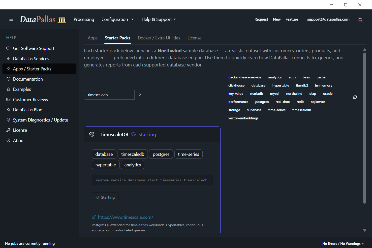
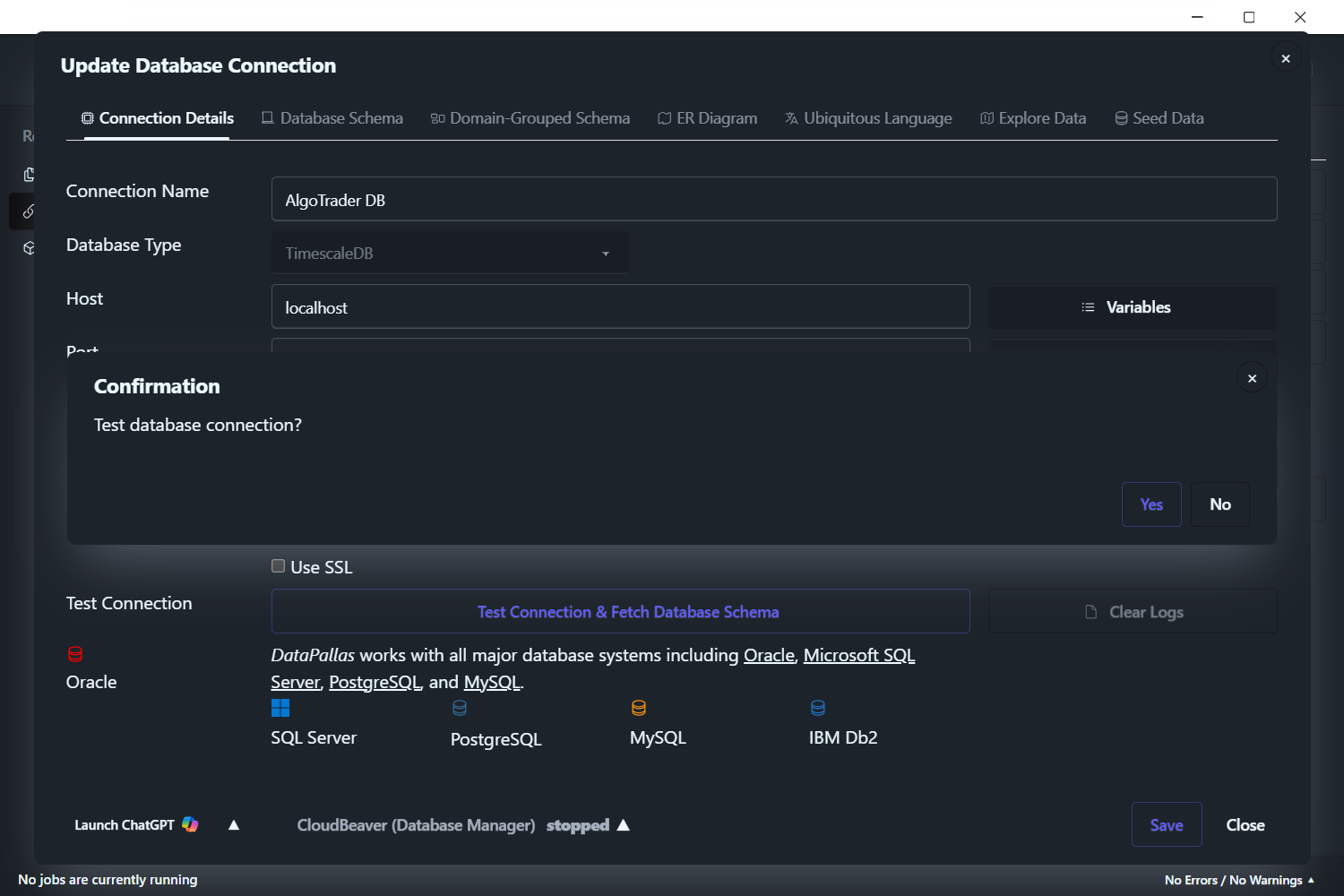
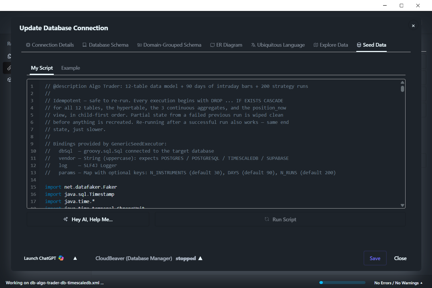
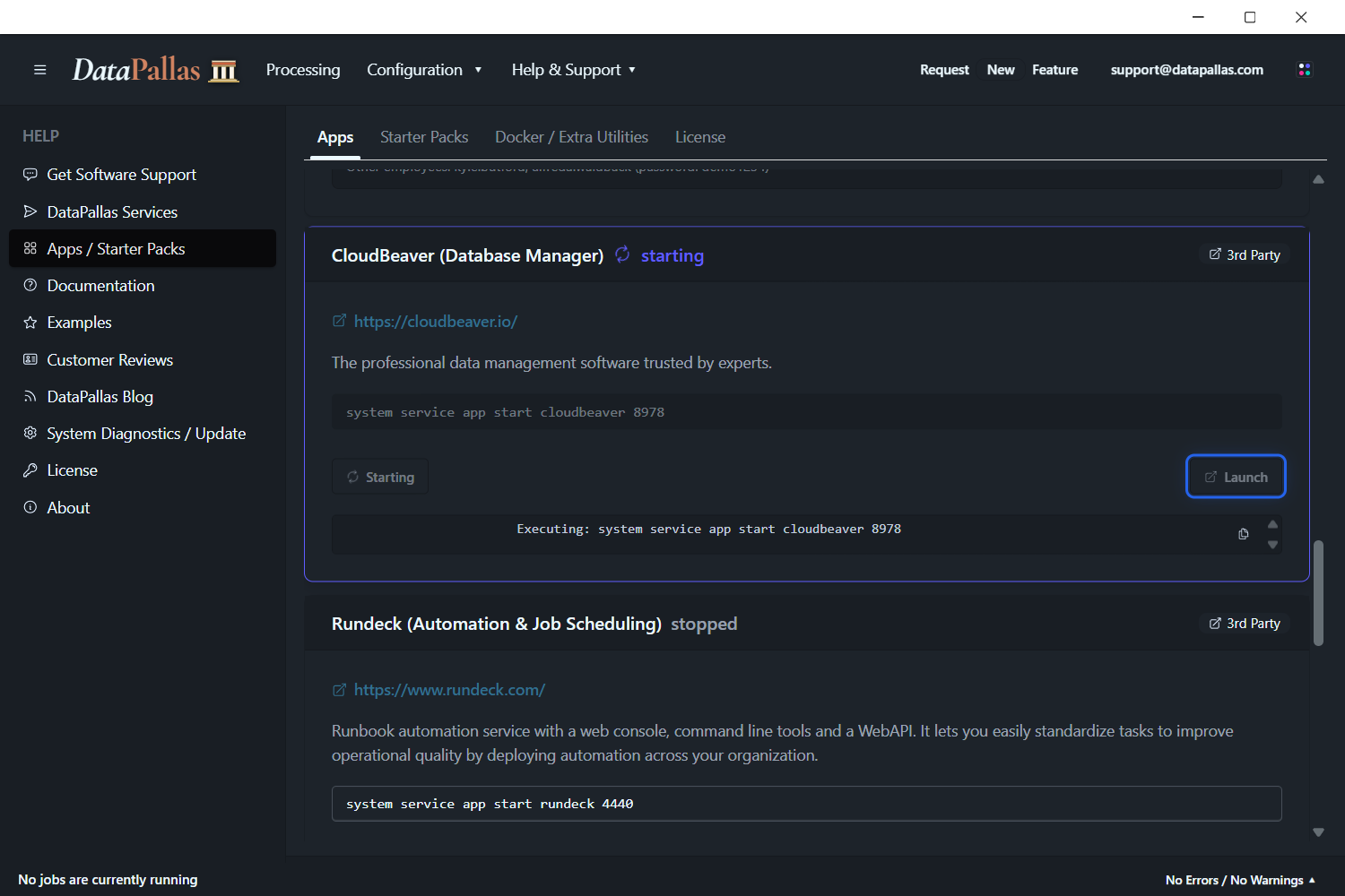
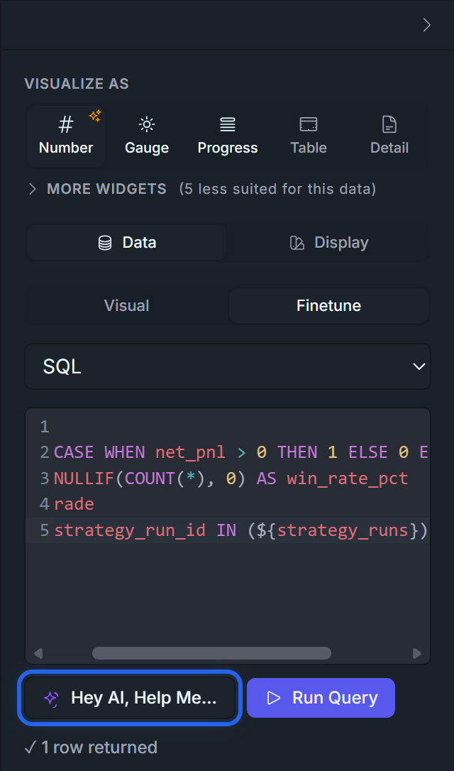
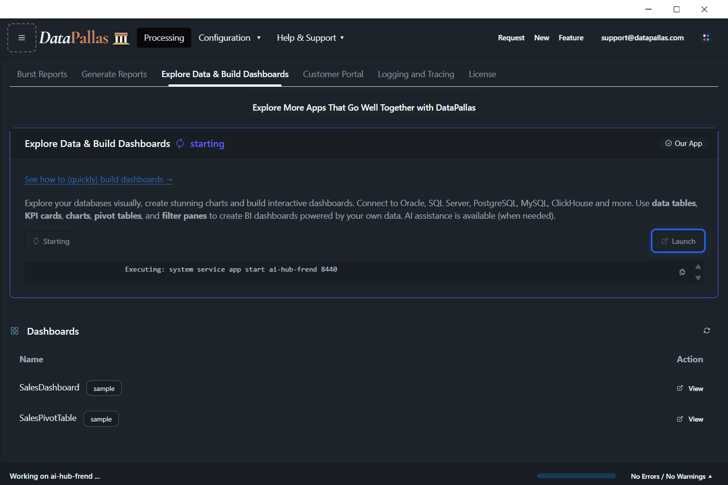

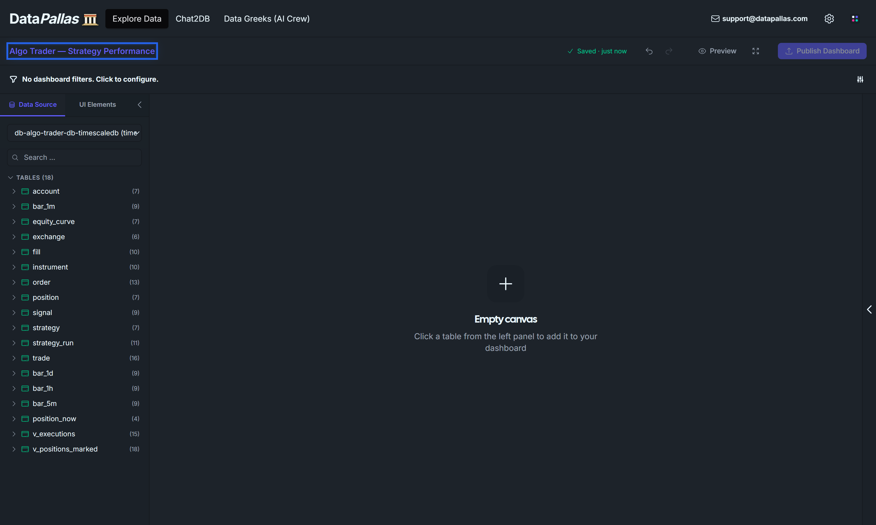
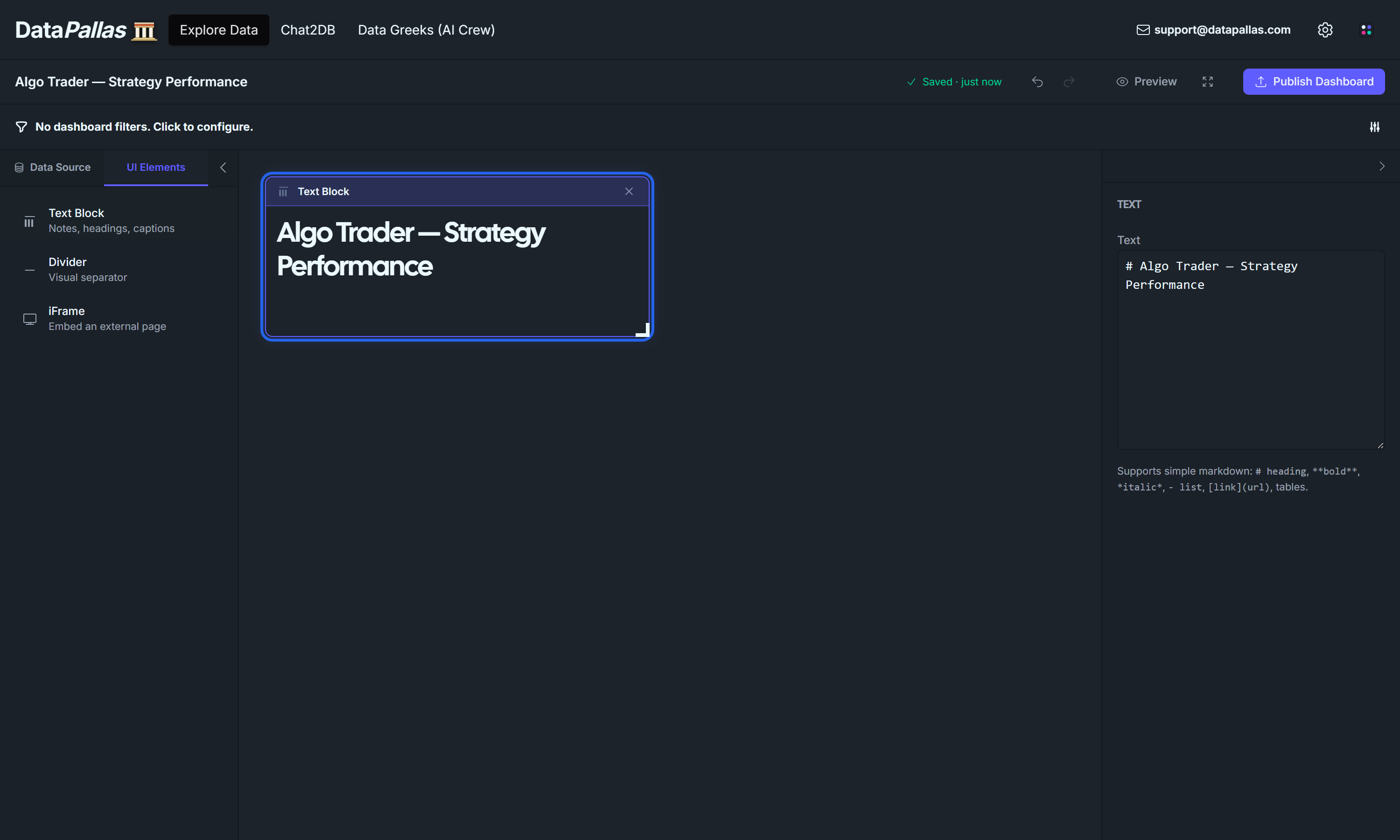
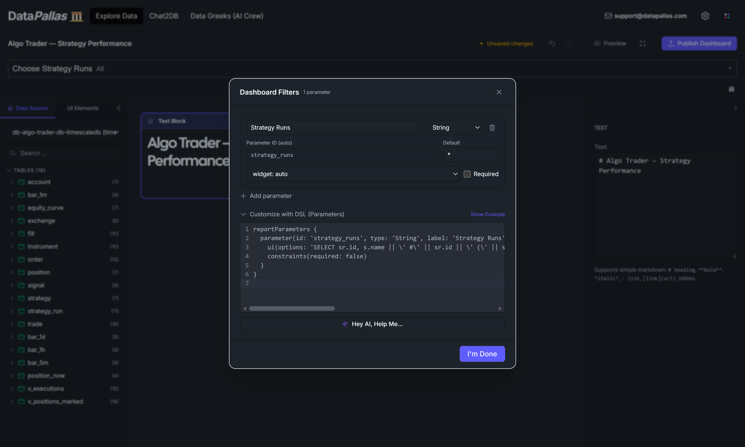
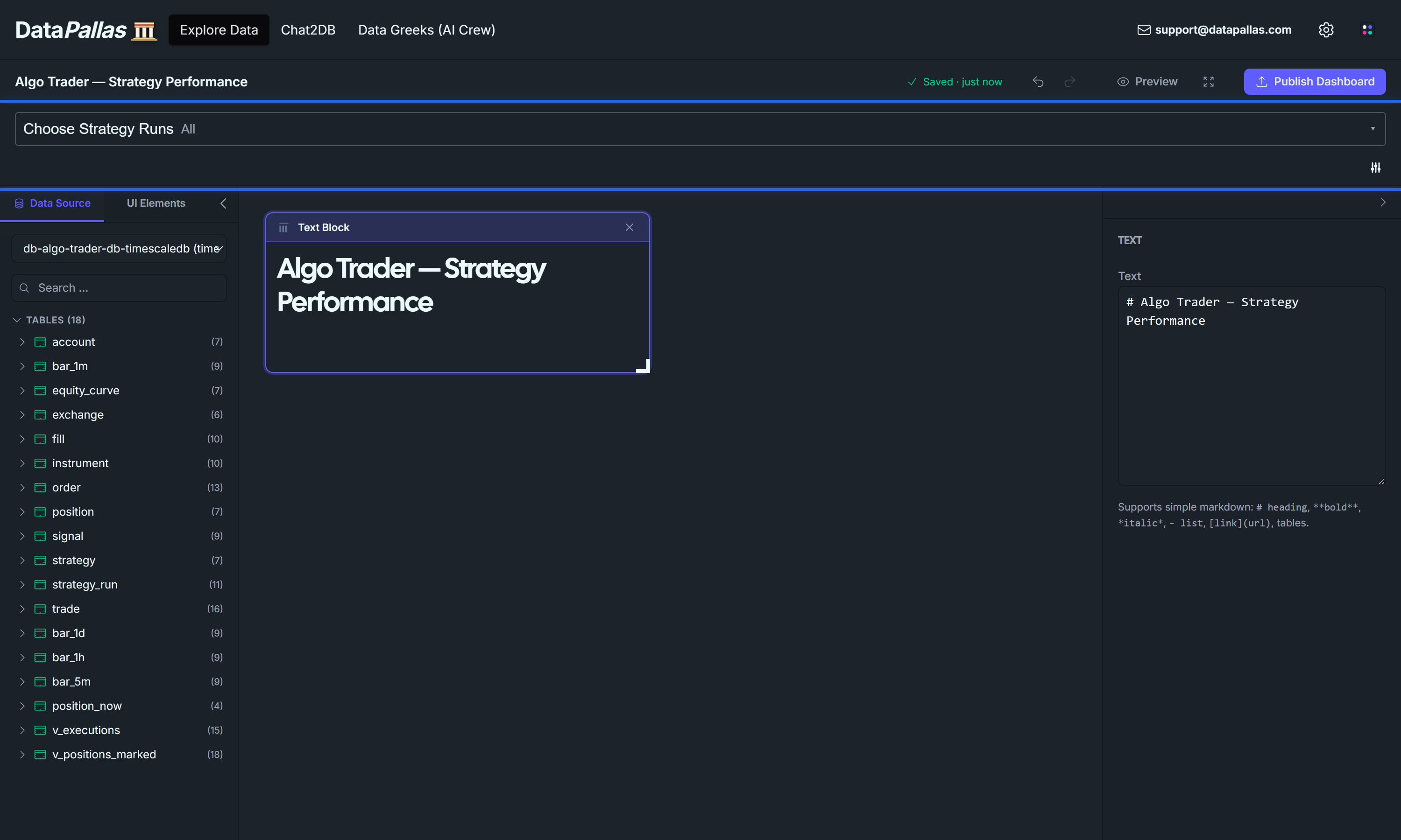
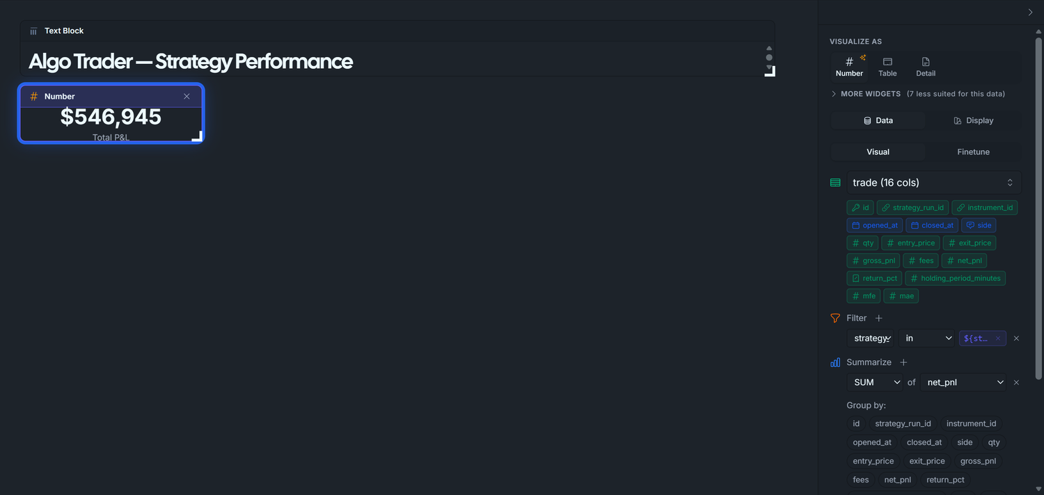
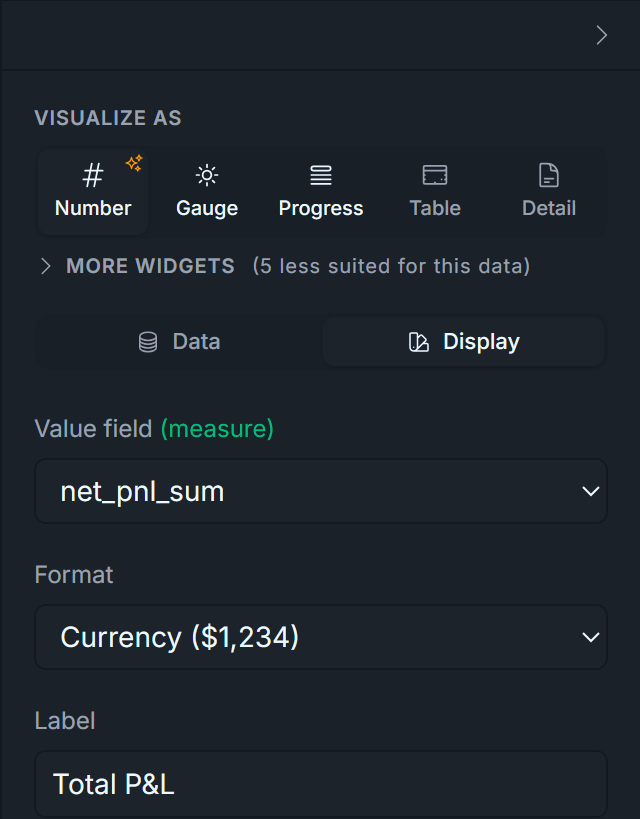
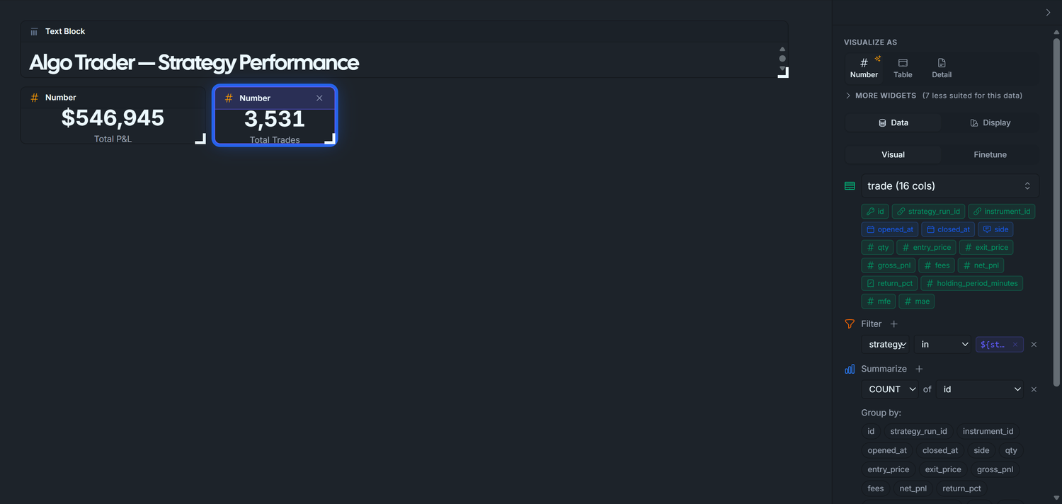
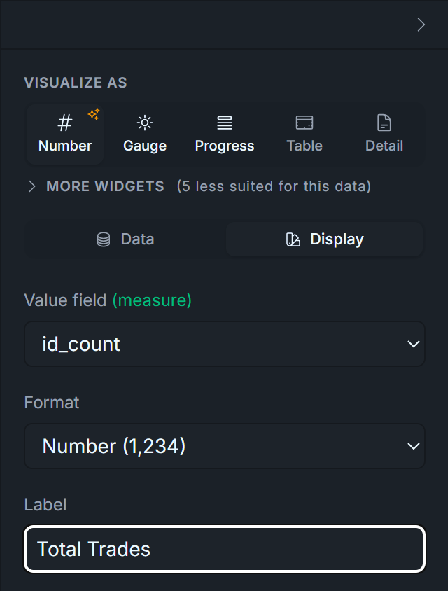
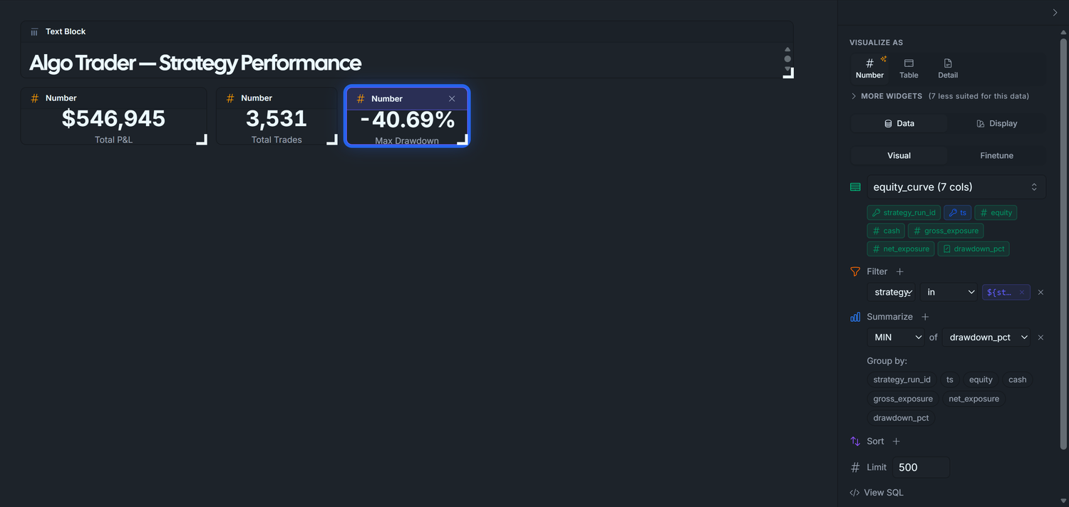
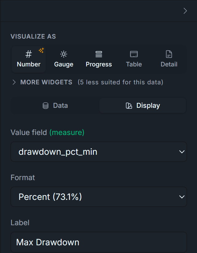
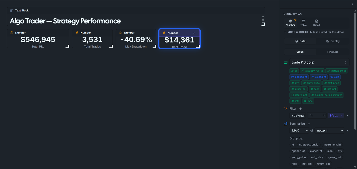
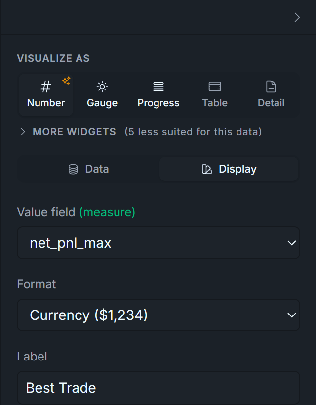
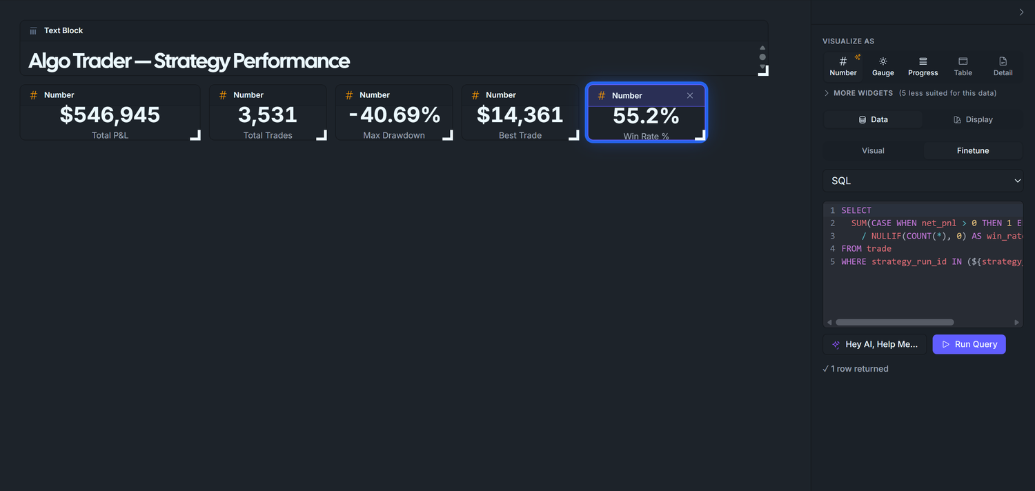
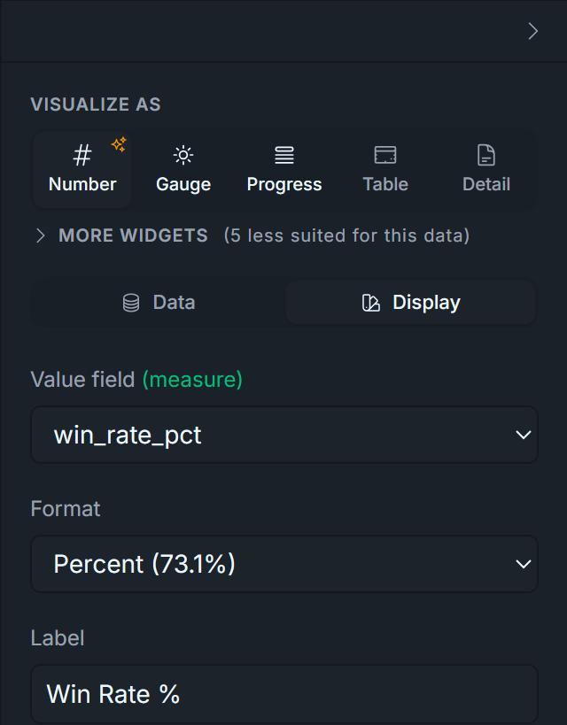
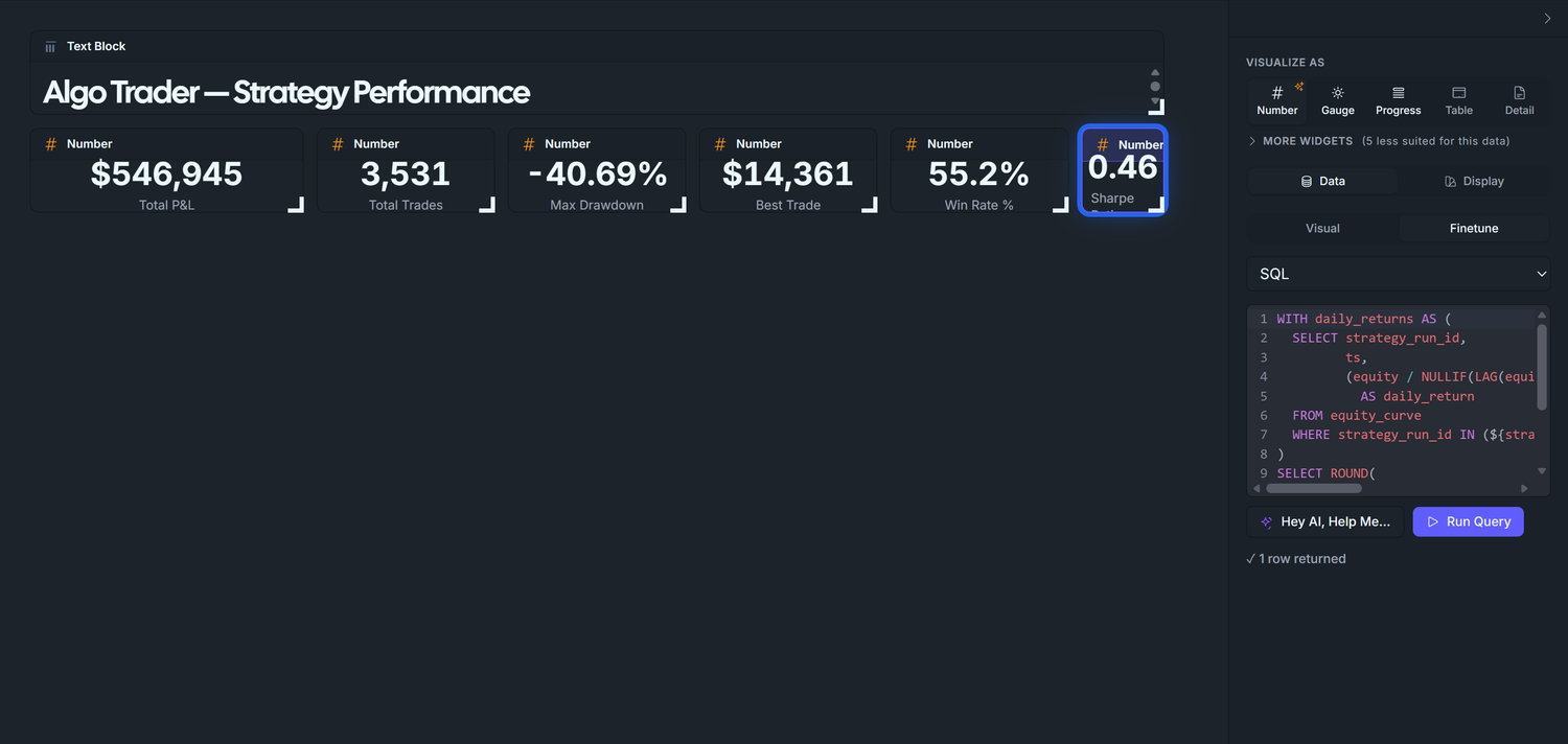
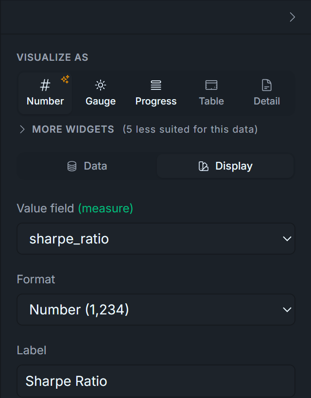
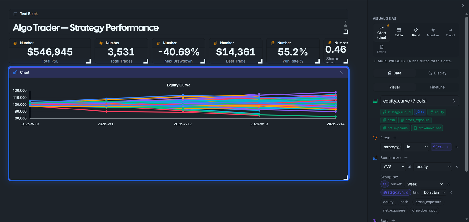
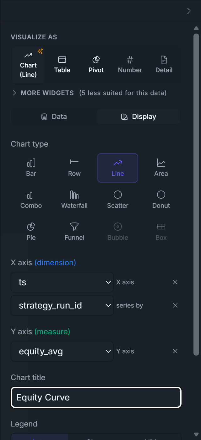
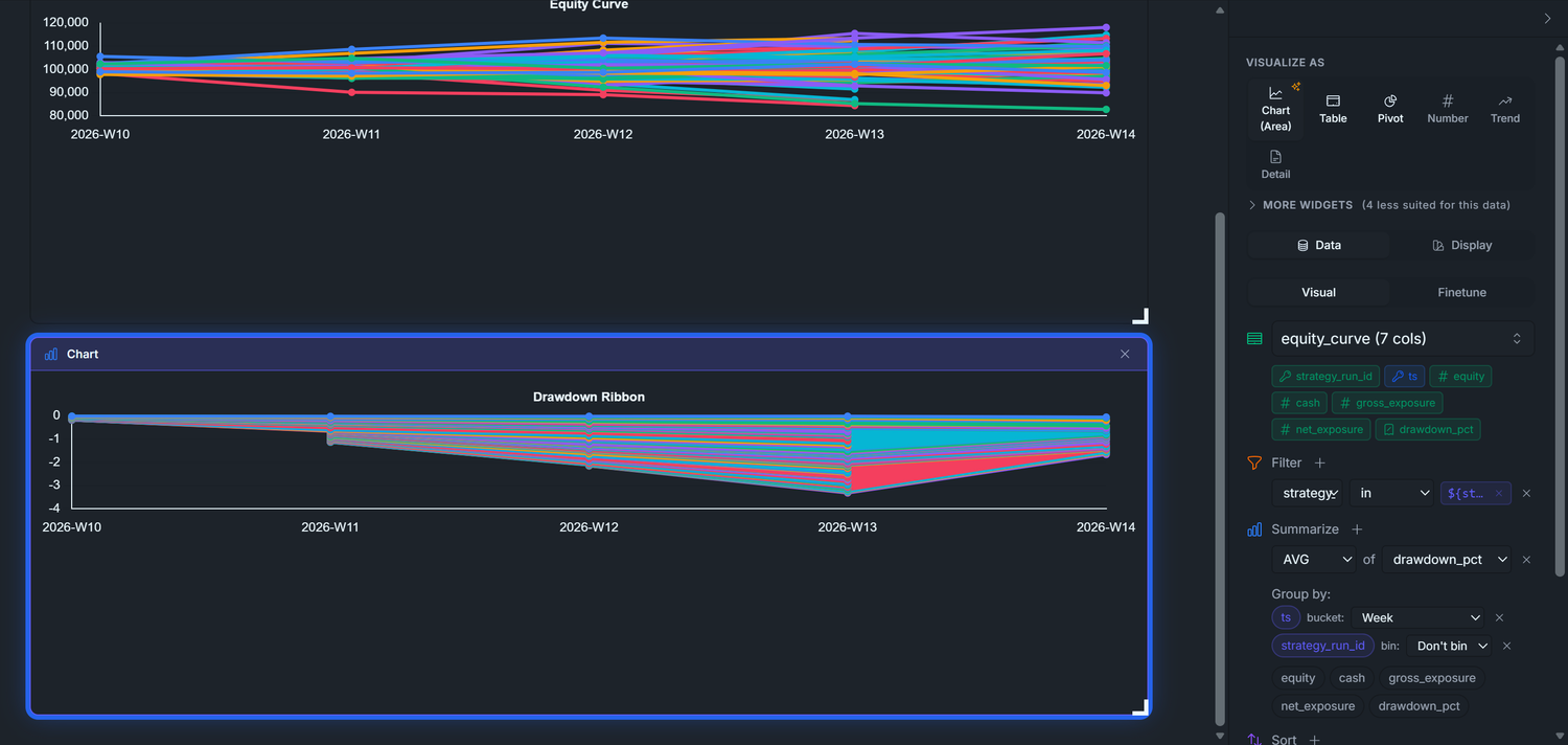
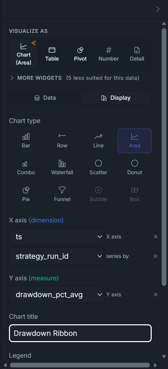

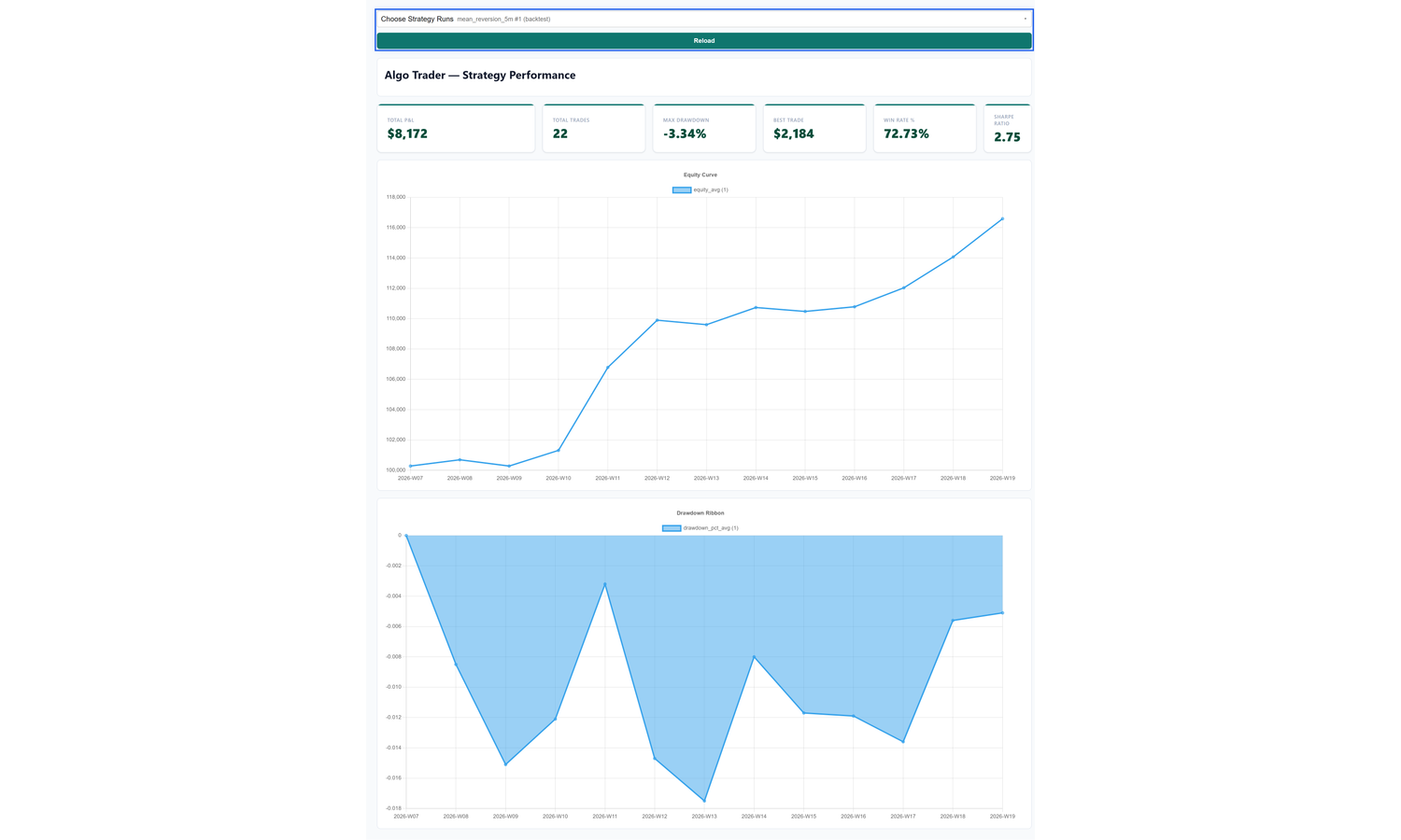

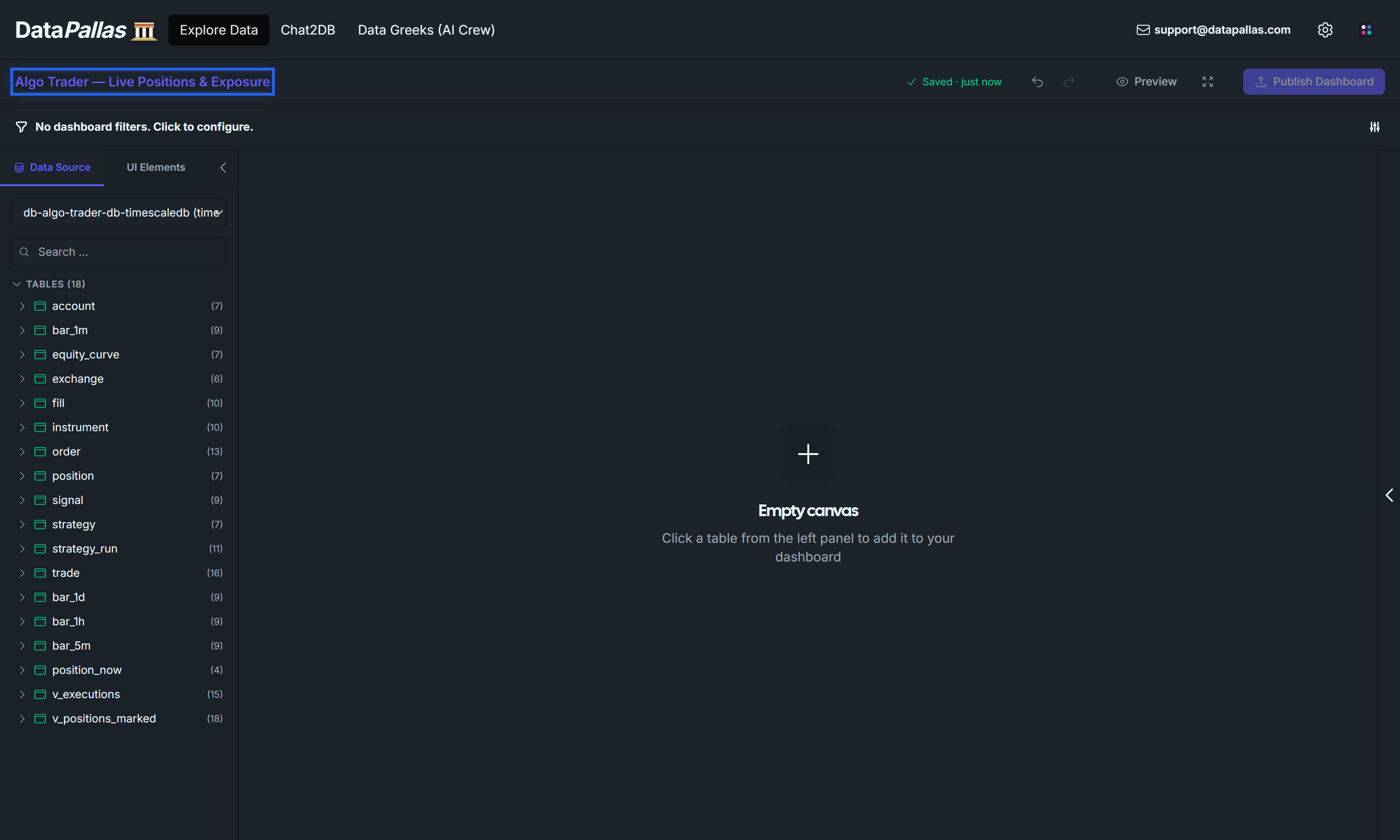
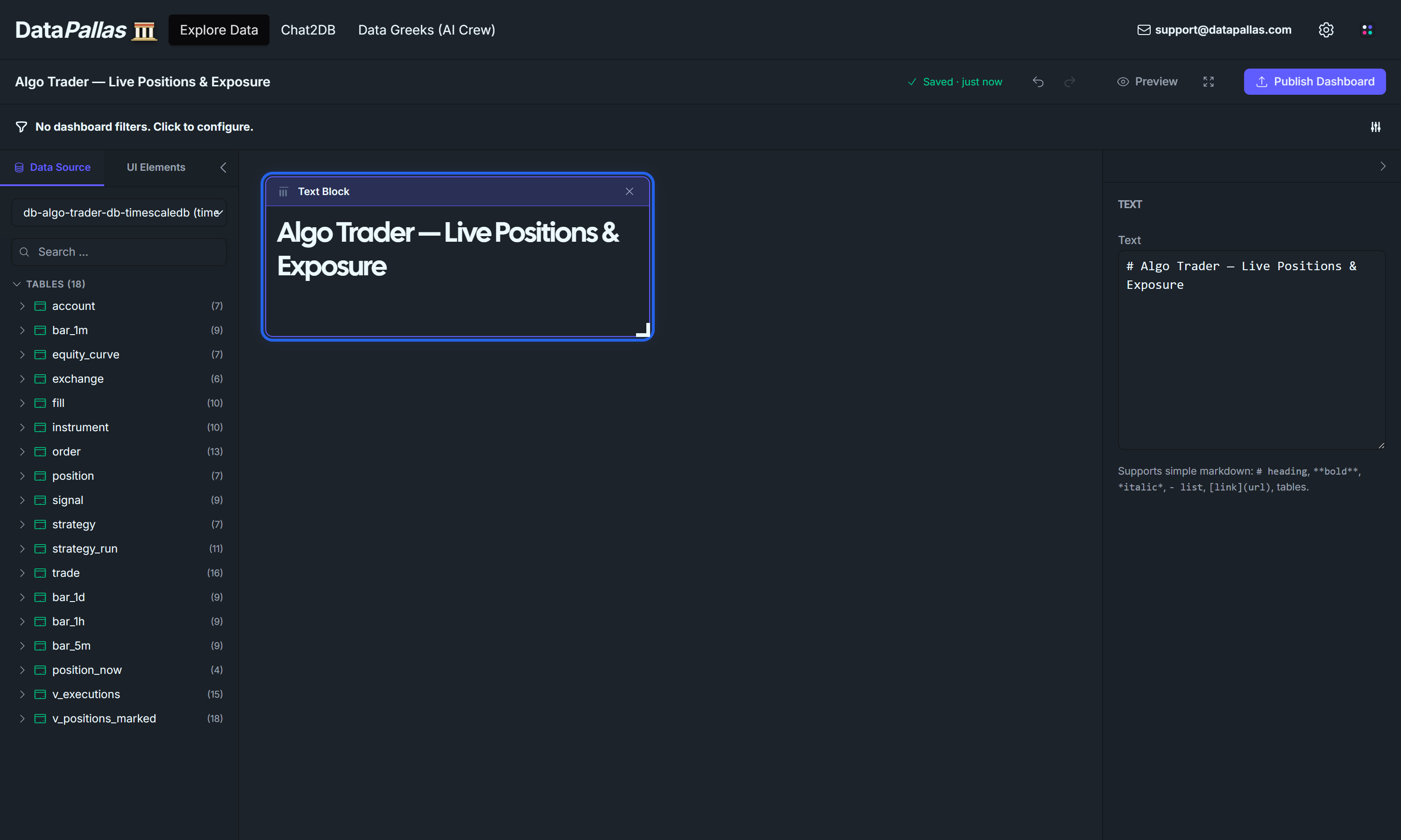
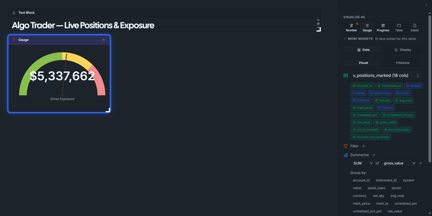
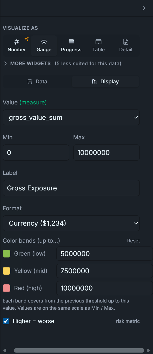
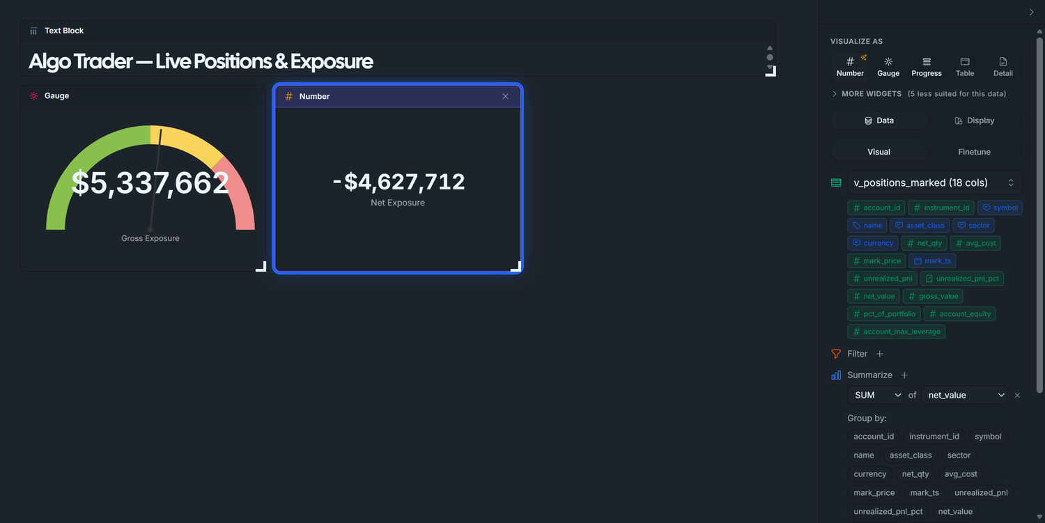
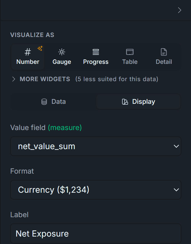
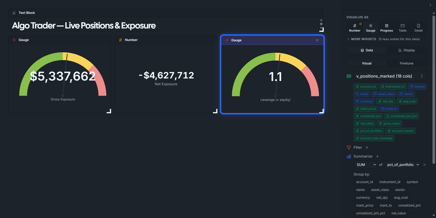
![Display tab — Leverage: Gauge widget with Min 0, Max 2, three bands [1, 1.5, 2] and Higher-is-worse on. — dark theme](/images/blog/algo-trading/034_d2-leverage-display-dark.png)